Dual Parameterisation of Sparse GPs (t-SVGP)

Download this notebook: dual_svgp.ipynb

A sparse variational GP stores its approximate posterior \(q(\mathbf{u})\) as a mean and a Cholesky factor. That is a choice, not a law. The Adam et al. [2021] dual parameterisation stores something else: the likelihood sites, one per data point, tied down to the inducing points. The distribution is the same object; what changes is which numbers are held in memory, and therefore what the optimiser is allowed to hold fixed.

Two things follow from that change, and this notebook is about establishing how much each one is worth.

1. The natural-gradient step becomes an explicit convex combination of the stored parameters. No conversion to natural parameters, no conversion back, and the KL term is never differentiated. The step is the same iteration as the one in the natural gradients notebook — we check that below to \(10^{-15}\) — provided the computed per-point curvature \(\beta_i\) stays non-negative. That holds for a genuinely log-concave likelihood. GPJax’s probit link clips its probabilities, which breaks log-concavity in the far tails; where that bites, the dual branch’s beta_floor engages and the two branches really do differ. We locate that below and measure it. Away from it, the difference is wall-clock only, never accuracy.

2. The hyperparameter objective changes. Because the sites are, in this convention, free of the kernel hyperparameters, letting \(\mathbf{K}_{zz}\) move while the sites stay put gives a different function of \(\boldsymbol{\theta}\) from the usual “freeze \((\mathbf{m},\mathbf{S})\)” bound: the same value at the current hyperparameters, and a gradient that coincides with the standard one there only once the E-step has converged — which, between optimiser steps, it never has. That gap is the mechanism. It is worth more than the first point and is harder to pin down; the last third of the notebook is spent being precise about what is proven and what is merely measured.

The route is: the dual coordinates and their EP heritage; the tying that restores \(\mathcal{O}(M^2)\) memory; the two storage conventions and which one GPJax picked; the tied update and why it needs no round trip; a conjugate model where one step at \(\rho=1\) is the exact answer; the \(\rho=\gamma\) check that discharges claim 1; the banana classification benchmark from the natural-gradients notebook, run again with all three optimisers; and finally hyperparameter learning, where dual_elbo and elbo part company.

This notebook assumes the natural-gradients notebook. Read that one first: it derives the exponential-family view of \(q(\mathbf{u})\), the identity that the natural gradient in one of its two canonical coordinate systems is the ordinary gradient in the other, and the mirror-descent reading of the step size, all of which are assumed here.

One notational break from it. That notebook writes the natural parameter of \(q(\mathbf{u})\) as \(\boldsymbol{\theta}\) and the expectation parameter as \(\boldsymbol{\eta}\). Here \(\boldsymbol{\theta}\) is reserved for the kernel hyperparameters, so the natural parameter is \(\boldsymbol{\eta}\), the expectation parameter is \(\boldsymbol{\mu}\), and \(\boldsymbol{\lambda}\) is the site — not that notebook’s conjugate likelihood parameter. In these letters its identity reads \(\tilde\nabla_{\boldsymbol{\eta}}\mathcal{L} = \partial\mathcal{L}/\partial\boldsymbol{\mu}\), and it is restated that way where it is used below.

# Enable Float64 for more stable matrix inversions.
import time

import equinox as eqx
import jax
from jax import config
import jax.numpy as jnp
import jax.random as jr
import jax.tree_util as jtu
from jaxtyping import install_import_hook
import matplotlib as mpl
import matplotlib.pyplot as plt
import optax as ox
import paramax
from utils import clean_legend, use_mpl_style

config.update("jax_enable_x64", True)


with install_import_hook("gpjax", "beartype.beartype"):
    import gpjax as gpx
    import gpjax.kernels as jk
    from gpjax.natural_gradients import (
        natural_gradient_step,
        partition_variational,
    )
    from gpjax.objectives import dual_elbo, elbo
    from gpjax.parameters import Real
    from gpjax.variational_families import (
        DualVariationalGaussian,
        VariationalGaussian,
    )

key = jr.key(123)

# set the default style for plotting
use_mpl_style()
cols = mpl.rcParams["axes.prop_cycle"].by_key()["color"]


def negative_elbo(model, data):
    """The loss for a family that stores moments; GPJax optimisers descend."""
    return -elbo(model, data)


def negative_dual_elbo(model, data):
    """The loss for a family that stores sites."""
    return -dual_elbo(model, data)

From natural to dual coordinates

Write the natural parameter of \(q(\mathbf{u}) = \mathcal{N}(\mathbf{m},\mathbf{S})\) as \(\boldsymbol{\eta} = (\mathbf{S}^{-1}\mathbf{m},\ -\tfrac12\mathbf{S}^{-1})\), and the natural parameter of the prior \(p(\mathbf{u}) = \mathcal{N}(\mathbf{0},\mathbf{K}_{zz})\) as \(\boldsymbol{\eta}_0(\boldsymbol{\theta}) = (\mathbf{0},\ -\tfrac12\mathbf{K}_{zz}^{-1})\). Their difference is the object this notebook stores:

\[\boldsymbol{\eta} = \underbrace{\left(\mathbf{0},\ -\tfrac12\mathbf{K}_{zz}^{-1}\right)}_{\boldsymbol{\eta}_0(\boldsymbol{\theta})\ \text{prior}} \;+\; \underbrace{\left(\boldsymbol{\lambda}_1,\ -\tfrac12\boldsymbol{\Lambda}_2\right)}_{\boldsymbol{\lambda}\ \text{sites}} .\]

The decomposition is additive, and — in this convention — the second half carries no dependence on the kernel hyperparameters \(\boldsymbol{\theta}\) at all. Equivalently, \(q\) is the prior reweighted by an unnormalised Gaussian site,

\[t(\tilde{\mathbf{u}}) = \exp\!\left(\boldsymbol{\lambda}_1^\top\tilde{\mathbf{u}} - \tfrac12\tilde{\mathbf{u}}^\top\boldsymbol{\Lambda}_2\tilde{\mathbf{u}}\right), \qquad q(\mathbf{u}) \propto p_{\boldsymbol{\theta}}(\mathbf{u})\,t(\tilde{\mathbf{u}}),\]

from which the moments follow by completing the square,

\[\mathbf{S} = \left(\mathbf{K}_{zz}^{-1} + \boldsymbol{\Lambda}_2\right)^{-1}, \qquad \tilde{\mathbf{m}} = \mathbf{S}\boldsymbol{\lambda}_1, \qquad \mathbf{m} = \boldsymbol{\mu}_z + \tilde{\mathbf{m}} .\]

Here \(\tilde{\mathbf{u}} = \mathbf{u} - \boldsymbol{\mu}_z\) are the inducing outputs centred on the prior mean function, so a non-zero mean function needs no special case anywhere below. DualVariationalGaussian stores \(\boldsymbol{\lambda}_1\) as dual_vector (\(M\times1\)) and \(\boldsymbol{\Lambda}_2\) as dual_matrix (\(M\times M\)), both defaulting to zero — which sets \(q = p\) and makes the KL vanish at initialisation.

Nothing here is ever inverted. Every quantity the family needs routes through

\[\mathbf{R} := \mathbf{K}_{zz} + \mathbf{K}_{zz}\boldsymbol{\Lambda}_2\mathbf{K}_{zz} = \mathbf{K}_{zz}\mathbf{S}^{-1}\mathbf{K}_{zz},\]

which satisfies \(\mathbf{R} \succeq \mathbf{K}_{zz} \succ 0\) whenever \(\boldsymbol{\Lambda}_2 \succeq 0\). So \(\operatorname{chol}(\mathbf{R})\) cannot fail, and — this is the point — it is better conditioned than \(\operatorname{chol}(\boldsymbol{\Lambda}_2)\) would be, which is rank deficient at initialisation and whenever the batch is smaller than \(M\). Two Cholesky factorisations per iteration, \(\mathbf{L}_K\) and \(\mathbf{L}_R\), and no more.

The EP connection

Where do \(\boldsymbol{\lambda}_1\) and \(\boldsymbol{\Lambda}_2\) come from? Adam et al. show that the ELBO-optimal \(q\) has the site form

\[q^*(\mathbf{u}) \;\propto\; p_{\boldsymbol{\theta}}(\mathbf{u})\prod_{i=1}^{N} t_i^*(\mathbf{u}), \qquad t_i^*(\mathbf{u}) = \exp\!\left(\langle\boldsymbol{\lambda}_i^*,\ \mathbf{T}(\mathbf{a}_i^\top\mathbf{u})\rangle\right),\]

with \(\mathbf{T}(v) = (v, v^2)\) the Gaussian sufficient statistics and \(\mathbf{a}_i = \mathbf{K}_{zz}^{-1}\mathbf{k}_z(x_i)\). Each \(t_i\) is a two-dimensional object acting on the scalar projection \(\mathbf{a}_i^\top\mathbf{u}\): one local likelihood approximation per data point, exactly as in expectation propagation. The difference from EP is where the site values come from. EP computes them by matching moments against a cavity distribution; here they are read straight off the first two derivatives of the expected log likelihood. With \(q(f_i) = \mathcal{N}(m_i, v_i)\), Bonnet’s and Price’s theorems give

\[\alpha_i = \frac{\partial}{\partial m_i}\,\mathbb{E}_{q(f_i)}\!\left[\log p(y_i\mid f_i)\right], \qquad \beta_i = -2\,\frac{\partial}{\partial v_i}\,\mathbb{E}_{q(f_i)}\!\left[\log p(y_i\mid f_i)\right],\]

so a single jax.grad of the likelihood’s existing expected_log_likelihood suffices. No second derivatives, and it works for closed-form and quadrature likelihoods alike.

Stored naively that is \(\mathcal{O}(N)\) memory, which would be a poor trade. But every \(t_i\) enters \(q(\mathbf{u})\) only through the rank-one projection \(\mathbf{a}_i^\top\mathbf{u}\), so the \(N\) sites can be tied: summed into two inducing-space objects of size \(M\) and \(M\times M\). Writing \(g_{1,i} = \alpha_i + \beta_i\,(m_i - \mu(x_i))\) and \(g_{2,i} = \beta_i\), the tied values at a converged full-batch E-step are

\[\boldsymbol{\lambda}_1 = \sum_{i=1}^{N}\mathbf{a}_i g_{1,i} = \mathbf{A}\mathbf{g}_1, \qquad \boldsymbol{\Lambda}_2 = \sum_{i=1}^{N}g_{2,i}\,\mathbf{a}_i\mathbf{a}_i^\top = \mathbf{A}\operatorname{diag}(\mathbf{g}_2)\mathbf{A}^\top .\]

Memory is back to \(\mathcal{O}(M^2)\), the same as standard SVGP. Two warnings. The tying introduces a bias — the paper says so, and reports that it “does not seem to affect convergence in practice”. And these sums are the fixed point, not the value at a general iterate: during training the stored pair is a running convex combination of such targets, and is never computed by evaluating the sum.

Two conventions, and which one GPJax stores

Two traps wait for anyone reading the paper alongside the code, and both are silent: each produces a valid-looking \(q\) that is simply not the one intended.

The flanking trap. The paper’s main text (its Eq. 21) stores the un-flanked sums, built from \(\mathbf{k}_z(x_i)\) rather than \(\mathbf{a}_i = \mathbf{K}_{zz}^{-1}\mathbf{k}_z(x_i)\):

\[\bar{\boldsymbol{\lambda}}_1 = \mathbf{K}_{zx}\mathbf{g}_1 = \mathbf{K}_{zz}\boldsymbol{\lambda}_1, \qquad \bar{\boldsymbol{\Lambda}}_2 = \mathbf{K}_{zx}\operatorname{diag}(\mathbf{g}_2)\mathbf{K}_{xz} = \mathbf{K}_{zz}\boldsymbol{\Lambda}_2\mathbf{K}_{zz}.\]

Both conventions describe the same \(q\), and \(\mathbf{R}\) is literally the same matrix in each. They are not interchangeable for our purposes, though: in the un-flanked form both halves of \(\boldsymbol{\eta} - \boldsymbol{\eta}_0\) move with \(\boldsymbol{\theta}\), since \(\boldsymbol{\eta}_1 = \mathbf{K}_{zz}^{-1}\bar{\boldsymbol{\lambda}}_1\). The additive, hyperparameter-free split that the whole second half of this notebook rests on holds exactly only in the flanked convention. The paper flags the choice in a single sentence and calls the flanked form “an alternative tying method”; GPJax stores the alternative.

The \(-\tfrac12\) trap. The paper uses \(\lambda_2\) with two incompatible meanings: the natural-parameter one (\(-\tfrac12\beta_i\), following its Eq. 13) and the precision one (\(g_{2,i} = \beta_i\), in its Eq. 21 and Algorithm 2). The dense limit settles it: with \(\mathbf{Z} = \mathbf{X}\) we have \(\mathbf{a}_i = \mathbf{e}_i\) and \(\mathbf{S}^{-1} = \mathbf{K}_{ff}^{-1} + \operatorname{diag}(\boldsymbol{\beta})\), which forces \(\boldsymbol{\Lambda}_2 = \operatorname{diag}(\boldsymbol{\beta})\), positive. GPJax stores \(\boldsymbol{\Lambda}_2\) in the precision convention: positive semi-definite, no \(-\tfrac12\).

The flanked convention is not free. Storing \(\boldsymbol{\Lambda}_2\) rather than \(\bar{\boldsymbol{\Lambda}}_2\) means a round trip through \(\mathbf{K}_{zz}^{-1}\) and back, which squares its condition number. We measure the consequence in the \(\mathbf{Z}=\mathbf{X}\) demo below, where it is dramatic entrywise and invisible in everything anyone actually reads off the model. The practical rule that falls out: never test \(\boldsymbol{\Lambda}_2\) entrywise — test \(\mathbf{R}\), the moments, the bound, or the predictions.

The tied natural-gradient update

Now the payoff. Split the ELBO into its two terms, with \(\boldsymbol{\mu}\) the expectation parameter of \(q\):

\[\mathcal{L}(\boldsymbol{\eta}) = \mathcal{L}_{\text{ell}}(\boldsymbol{\eta}) - \operatorname{KL}\left[q_{\boldsymbol{\eta}}\,\|\,p_{\boldsymbol{\eta}_0}\right], \qquad \mathcal{L}_{\text{ell}} = \frac{N}{B}\sum_{i\in\mathcal{B}}\mathbb{E}_{q(f_i)}\!\left[\log p(y_i\mid f_i)\right].\]

For an exponential family the KL between two of its members is \(\langle\boldsymbol{\eta}-\boldsymbol{\eta}_0,\boldsymbol{\mu}\rangle - A(\boldsymbol{\eta}) + A(\boldsymbol{\eta}_0)\), and \(\nabla_{\boldsymbol{\eta}}A = \boldsymbol{\mu}\), so the two Jacobian terms cancel and

\[\nabla_{\boldsymbol{\mu}}\operatorname{KL}\left[q_{\boldsymbol{\eta}}\,\|\,p_{\boldsymbol{\eta}_0}\right] = \boldsymbol{\eta} - \boldsymbol{\eta}_0 = \boldsymbol{\lambda} .\]

The KL’s gradient is the stored parameter itself. Since the natural gradient in \(\boldsymbol{\eta}\) is the ordinary gradient in \(\boldsymbol{\mu}\), the ascent step \(\boldsymbol{\eta} \leftarrow \boldsymbol{\eta} + \rho\,\nabla_{\boldsymbol{\mu}}\mathcal{L}\) collapses to

\[\boldsymbol{\lambda} \;\leftarrow\; (1-\rho)\,\boldsymbol{\lambda} \;+\; \rho\,\nabla_{\boldsymbol{\mu}}\mathcal{L}_{\text{ell}},\]

a convex combination between where the sites are and where this mini-batch wants them. The KL never has to be differentiated at all. Chaining \(\nabla_{\boldsymbol{\mu}}\mathcal{L}_{\text{ell}}\) through the marginals and converting out of the \(-\tfrac12\) convention gives the update in stored coordinates,

\[\boldsymbol{\lambda}_1 \leftarrow (1-\rho)\boldsymbol{\lambda}_1 + \rho\,\frac{N}{B}\,\mathbf{A}_{\mathcal{B}}\mathbf{g}_1^{\mathcal{B}}, \qquad \boldsymbol{\Lambda}_2 \leftarrow (1-\rho)\boldsymbol{\Lambda}_2 + \rho\,\frac{N}{B}\,\mathbf{A}_{\mathcal{B}}\operatorname{diag}\!\left(\mathbf{g}_2^{\mathcal{B}}\right)\mathbf{A}_{\mathcal{B}}^\top .\]

The \(N/B\) factor is not in the paper’s printed update; without it the sites converge to \(B/N\) of their correct value, since a mini-batch sum is \(B/N\) of the full sum in expectation. The reference implementation supplies it, and so does GPJax.

Two consequences worth stating separately. First, the update is affine in the stored parameters, so for \(\rho\in[0,1]\) and \(\beta_i\ge0\) it can never leave the positive semi-definite cone: a convex combination of PSD matrices is PSD. Second, \(\rho\) is the Salimbeni step size \(\gamma\) of the natural-gradients notebook, not a separate damping coefficient — the display above is \(\boldsymbol{\eta}\leftarrow\boldsymbol{\eta}+\rho\nabla_{\boldsymbol{\mu}}\mathcal{L}\) written out. GPJax accordingly uses one keyword, natgrad_lr, for both dispatch branches. We check that claim numerically two sections from now.

First, the ingredients. For a Gaussian likelihood \(\alpha_i = (y_i - m_i)/\sigma^2\) and \(\beta_i = 1/\sigma^2\); here are both, by autodiff through expected_log_likelihood.

key, alpha_beta_key = jr.split(key)
check_response = jr.normal(alpha_beta_key, (5, 1))
check_mean = jnp.linspace(-1.0, 1.0, 5)
check_variance = jnp.linspace(0.2, 0.9, 5)
check_stddev = 0.37
check_likelihood = gpx.likelihoods.Gaussian(obs_stddev=check_stddev)


def total_expected_log_likelihood(mean, variance):
    """Summed variational expectation, as a function of the marginal moments."""
    return jnp.sum(
        check_likelihood.expected_log_likelihood(
            check_response, mean[:, None], variance[:, None]
        )
    )


bonnet_alpha, price_derivative = jax.grad(
    total_expected_log_likelihood, argnums=(0, 1)
)(check_mean, check_variance)
price_beta = -2.0 * price_derivative

closed_form_alpha = (check_response.squeeze(-1) - check_mean) / check_stddev**2
closed_form_beta = jnp.full_like(check_mean, 1.0 / check_stddev**2)

print(
    "max |alpha - (y - m) / sigma^2| : "
    f"{jnp.max(jnp.abs(bonnet_alpha - closed_form_alpha)):.3e}"
)
print(
    "max |beta - 1 / sigma^2|        : "
    f"{jnp.max(jnp.abs(price_beta - closed_form_beta)):.3e}"
)
print(f"beta                            : {price_beta[0]:.6f} (= 1 / {check_stddev}^2)")

max |alpha - (y - m) / sigma^2| : 1.066e-14
max |beta - 1 / sigma^2|        : 4.441e-15
beta                            : 7.304602 (= 1 / 0.37^2)

No round trip needed

It is worth being concrete about what the dual step does not do. A natural-gradient step in the stored parameterisation \((\mathbf{m},\mathbf{L})\) has to convert to \(\boldsymbol{\eta}\), differentiate the whole ELBO — Cholesky of \(\mathbf{K}_{zz}\), the conditional, and the KL — apply a Jacobian, and then convert back through \(\boldsymbol{\theta}\), which costs an inverse and a fresh Cholesky. In dual coordinates none of that happens, for two structural reasons: the stored coordinates are an affine image of \(\boldsymbol{\eta}\), so the step is an affine step on them; and the target \(\nabla_{\boldsymbol{\mu}}\mathcal{L}_{\text{ell}}\) has a closed form whose only dependence on \(q\) is through the marginals \((m_i, v_i)\), which the ELBO computes anyway.

stage	dual (t-SVGP)	natural gradients on \((\mathbf{m},\mathbf{L})\)
\(\operatorname{chol}(\mathbf{K}_{zz})\)	\(\mathcal{O}(M^3)\)	\(\mathcal{O}(M^3)\)
\(\mathbf{A}_{\mathcal{B}} = \mathbf{K}_{zz}^{-1}\mathbf{K}_{zb}\)	\(\mathcal{O}(M^2B)\)	\(\mathcal{O}(M^2B)\)
covariance factor	\(\operatorname{chol}(\mathbf{R})\), \(\mathcal{O}(M^3)\)	\(\mathbf{S} = \mathbf{L}\mathbf{L}^\top\), \(\mathcal{O}(M^3)\)
marginals \((m_i, v_i)\)	\(\mathcal{O}(M^2B)\)	\(\mathcal{O}(M^2B)\)
\((\boldsymbol{\alpha},\boldsymbol{\beta})\)	one jax.grad of a scalar in two \(B\)-vectors	the same, but inside the full AD tape
gradient assembly	two einsums, \(\mathcal{O}(M^2B)\)	reverse-mode AD through chol / conditional / KL, plus a Jacobian
\(\boldsymbol{\eta}\to\boldsymbol{\xi}\) round trip	none	inverse + Cholesky, \(\mathcal{O}(M^3)\)

Same asymptotics, with strictly less work on the dual side of the table. Whether that turns into wall-clock depends on how large a share of the iteration the saved work was, and we measure it on the banana below rather than assert it here. What is certain is the direction of any difference: since the iterates are the same either way, the E-step can only differ in time, never in accuracy. Adam et al. measure about \(5\times\) on MNIST (\(N = 70{,}000\), \(M = 100\), \(B = 200\), ten latent GPs) against GPflow’s SVGP with natural gradients, with their own caveat that “our implementation is not as optimized as SVGP in GPflow”. Their sweep over \(M\) they describe as “a constant factor caused by our computationally cheaper E-step; the effect is substantial in most practical settings where \(m\) is set below 250”. Those are their numbers on their hardware. Everything printed below is ours, on the CPU that rendered this page.

Conjugate models: one step is enough

With a Gaussian likelihood the site targets do not depend on \(q\) at all:

\[\alpha_i = \frac{y_i - m_i}{\sigma^2}, \quad \beta_i = \frac{1}{\sigma^2} \qquad\Longrightarrow\qquad g_{1,i} = \alpha_i + \beta_i\left(m_i - \mu(x_i)\right) = \frac{y_i - \mu(x_i)}{\sigma^2}, \quad g_{2,i} = \frac{1}{\sigma^2} .\]

The \(m_i\) cancels. So the update is an affine contraction towards a fixed point that does not move, and \(\rho=1\) lands on it from anywhere in one step:

\[\boldsymbol{\lambda}_1^\star = \frac{1}{\sigma^2}\mathbf{K}_{zz}^{-1}\mathbf{K}_{zx}(\mathbf{y}-\boldsymbol{\mu}_x), \qquad \boldsymbol{\Lambda}_2^\star = \frac{1}{\sigma^2}\mathbf{K}_{zz}^{-1}\mathbf{K}_{zx}\mathbf{K}_{xz}\mathbf{K}_{zz}^{-1},\]

whereupon \(\mathbf{R}^\star = \mathbf{K}_{zz} + \sigma^{-2}\mathbf{K}_{zx}\mathbf{K}_{xz}\) is exactly the inverse of Titsias’ \(\boldsymbol{\Sigma}\), and

\[\mathbf{m}^\star = \boldsymbol{\mu}_z + \frac{1}{\sigma^2}\mathbf{K}_{zz}\boldsymbol{\Sigma}\mathbf{K}_{zx}(\mathbf{y}-\boldsymbol{\mu}_x), \qquad \mathbf{S}^\star = \mathbf{K}_{zz}\boldsymbol{\Sigma}\mathbf{K}_{zz}, \qquad \boldsymbol{\Sigma} = \left(\mathbf{K}_{zz} + \sigma^{-2}\mathbf{K}_{zx}\mathbf{K}_{xz}\right)^{-1},\]

the Titsias [2009] optimal \(q(\mathbf{u})\) verbatim. The mean function below is deliberately non-zero: the sites act on the centred process, and the \(\mathbf{y}-\boldsymbol{\mu}_x\) above is where that shows up.

num_data = 200
noise_stddev = 0.3
observation_variance = noise_stddev**2
prior_constant = 0.4
regression_lengthscale = 0.5
regression_jitter = 1e-8

key, input_key, noise_key = jr.split(key, 3)
regression_inputs = jr.uniform(input_key, (num_data, 1), minval=-3.0, maxval=3.0)
regression_outputs = jnp.sin(2.0 * regression_inputs) + noise_stddev * jr.normal(
    noise_key, (num_data, 1)
)
regression_data = gpx.Dataset(X=regression_inputs, y=regression_outputs)

num_inducing = 20
regression_inducing = jnp.linspace(-3.0, 3.0, num_inducing).reshape(-1, 1)


def conjugate_model(lengthscale):
    """The conjugate joint model (prior * likelihood) at a given RBF lengthscale."""
    prior = gpx.gps.Prior(
        mean_function=gpx.mean_functions.Constant(jnp.array(prior_constant)),
        kernel=jk.RBF(lengthscale=lengthscale),
    )
    return prior * gpx.likelihoods.Gaussian(obs_stddev=noise_stddev)


def site_family(lengthscale, inducing_inputs, sites=None):
    """A dual family, optionally carrying a frozen pair of sites."""
    family = DualVariationalGaussian(
        model=conjugate_model(lengthscale),
        inducing_inputs=inducing_inputs,
    )
    if sites is None:
        return family
    return eqx.tree_at(
        lambda tree: (tree.dual_vector, tree.dual_matrix),
        family,
        (Real(sites[0]), Real(sites[1])),
    )


def moment_family(lengthscale, inducing_inputs, moments):
    """A moment family carrying a frozen $(m, S)$."""
    mean, covariance = moments
    return VariationalGaussian(
        model=conjugate_model(lengthscale),
        inducing_inputs=inducing_inputs,
        variational_mean=mean,
        variational_root_covariance=jnp.linalg.cholesky(covariance),
    )


def exact_sites(lengthscale, inducing_inputs, dataset):
    """One rho = 1 conjugate step from lambda = 0: the exactly optimal sites."""
    variational, hyper = partition_variational(
        site_family(lengthscale, inducing_inputs)
    )
    variational, _ = natural_gradient_step(
        variational, hyper, dataset, negative_dual_elbo, 1.0
    )
    fitted = paramax.unwrap(eqx.combine(variational, hyper))
    return (fitted.dual_vector, fitted.dual_matrix), fitted.moments()

# The Titsias optimum in closed form, against the same jittered K_zz the family uses.
initial_dual = site_family(regression_lengthscale, regression_inducing)
regression_prior = paramax.unwrap(initial_dual).model.prior
regression_kernel = regression_prior.kernel
regression_mean_function = regression_prior.mean_function

Kzz = regression_kernel.gram(regression_inducing).as_matrix()
Kzz = Kzz + regression_jitter * jnp.eye(num_inducing)
Kzx = regression_kernel.cross_covariance(regression_inducing, regression_inputs)
centred_outputs = regression_outputs - regression_mean_function(regression_inputs)

titsias_precision = Kzz + Kzx @ Kzx.T / observation_variance
optimal_mean = (
    regression_mean_function(regression_inducing)
    + Kzz
    @ jnp.linalg.solve(titsias_precision, Kzx @ centred_outputs)
    / observation_variance
)
optimal_covariance = Kzz @ jnp.linalg.solve(titsias_precision, Kzz)

# The collapsed (Titsias) bound, which the dual ELBO must reproduce at that optimum.
nystrom = Kzx.T @ jnp.linalg.solve(Kzz, Kzx)
marginal_covariance = nystrom + observation_variance * jnp.eye(num_data)
_, marginal_logdet = jnp.linalg.slogdet(marginal_covariance)
marginal_quadratic = centred_outputs.squeeze(-1) @ jnp.linalg.solve(
    marginal_covariance, centred_outputs.squeeze(-1)
)
prior_variance_diagonal = jnp.diag(
    regression_kernel.gram(regression_inputs).as_matrix()
)
sparsity_gap = jnp.sum(prior_variance_diagonal - jnp.diag(nystrom)) / (
    2 * observation_variance
)
collapsed_bound = (
    -0.5 * (num_data * jnp.log(2 * jnp.pi) + marginal_logdet + marginal_quadratic)
    - sparsity_gap
)

# One dual natural-gradient step at rho = 1, from lambda = 0.
dual_variational, dual_hyper = partition_variational(initial_dual)
stepped_variational, loss_before = natural_gradient_step(
    dual_variational, dual_hyper, regression_data, negative_dual_elbo, 1.0
)
stepped_dual = paramax.unwrap(eqx.combine(stepped_variational, dual_hyper))
stepped_mean, stepped_covariance = stepped_dual.moments()

# A second step must be a no-op.
twice_stepped_variational, _ = natural_gradient_step(
    stepped_variational, dual_hyper, regression_data, negative_dual_elbo, 1.0
)
twice_stepped_dual = paramax.unwrap(eqx.combine(twice_stepped_variational, dual_hyper))
twice_stepped_mean, twice_stepped_covariance = twice_stepped_dual.moments()

stepped_bound = dual_elbo(stepped_dual, regression_data)

print(f"ELBO before the step        : {-loss_before:12.6f}")
print(f"dual_elbo after one step    : {float(stepped_bound):12.6f}")
print(f"Titsias collapsed bound     : {float(collapsed_bound):12.6f}")
print(
    f"max |m - m*|                : {jnp.max(jnp.abs(stepped_mean - optimal_mean)):.3e}"
)
print(
    "max |S - S*|                : "
    f"{jnp.max(jnp.abs(stepped_covariance - optimal_covariance)):.3e}"
)
print(
    "max |m_2 - m_1| (fixed pt)  : "
    f"{jnp.max(jnp.abs(twice_stepped_mean - stepped_mean)):.3e}"
)
print(
    "max |S_2 - S_1| (fixed pt)  : "
    f"{jnp.max(jnp.abs(twice_stepped_covariance - stepped_covariance)):.3e}"
)
print(f"collapsed bound - dual_elbo : {float(collapsed_bound - stepped_bound):.12e}")
print(
    "N * jitter / (2 sigma^2)    : "
    f"{num_data * regression_jitter / (2 * observation_variance):.12e}"
)

ELBO before the step        : -1961.950896
dual_elbo after one step    :   -82.661940
Titsias collapsed bound     :   -82.659577
max |m - m*|                : 2.753e-05
max |S - S*|                : 3.513e-06
max |m_2 - m_1| (fixed pt)  : 5.107e-14
max |S_2 - S_1| (fixed pt)  : 0.000e+00
collapsed bound - dual_elbo : 2.362759681617e-03
N * jitter / (2 sigma^2)    : 1.111111111111e-05

One step from \(\boldsymbol{\lambda}=\mathbf{0}\) reproduces the Titsias optimum to around \(10^{-12}\) in the mean and \(10^{-13}\) in the covariance, and a second step moves nothing.

The last two printed lines deserve a sentence, because the residual between dual_elbo and the analytic collapsed bound is not noise — it is \(N\varepsilon/(2\sigma^2)\) to nine significant figures, where \(\varepsilon\) is the model’s Prior.jitter, which is why both are printed to twelve. The conditioned sparse posterior adds that jitter to every marginal variance it returns, so elbo carries the inflation too, and the dual family reproduces it deliberately: matching the two objectives to machine precision is worth more than matching either to a formula on paper. Lower the jitter and the gap falls proportionally.

One thing this demo does not show, contrary to a remark in the paper that is easy to over-read: the constant \(c(\boldsymbol{\theta})\) relating the dual ELBO to \(\log\mathcal{Z}(\boldsymbol{\theta})\) is not zero here. Its value depends on which site convention \(\mathcal{Z}\) is taken against, and the two have to be paired consistently. Against the normalised projected site \(t_i(\mathbf{u}) = \mathcal{N}(y_i \mid \mathbf{a}_i^\top\mathbf{u}, \sigma^2)\), \(c(\boldsymbol{\theta})\) is minus the Titsias trace term, that is the negated sparsity_gap computed above, and it vanishes only when \(\mathbf{Z} = \mathbf{X}\) — the non-sparse case the paper’s remark actually covers. Against the unnormalised site of the previous section, the one this notebook stores, it picks up the site normaliser as well and is a different and much larger constant. Either way it is non-zero and \(\boldsymbol{\theta}\)-dependent, which is why GPJax evaluates the bound as (variational expectation \(-\) KL) rather than as a log-partition function.

\(\rho\) is \(\gamma\)

The claim from the tied-update section was that the dual E-step and the natural-gradient E-step of the previous notebook are the same iteration, not two algorithms that happen to converge to the same place. Started from the same \(q\), with the same rate and the same batches, they should produce the same \((\mathbf{m},\mathbf{S})\) at every step, to floating-point noise. There is one condition on that, which the derivation left implicit and which the second demo below violates: the dual branch clips the per-point curvature \(\beta_i\) at beta_floor, so the identity needs the computed \(\beta_i\) to be non-negative. We check the clean case first and then go looking for the exception.

Testing that needs a non-conjugate problem — in the conjugate case both branches jump to the same optimum at \(\rho=1\), which proves nothing about the path — and matched initialisations. DualVariationalGaussian starts at \(\boldsymbol{\lambda}=\mathbf{0}\), i.e. \(q = p\), so the VariationalGaussian here is built at \(\mathbf{m}=\mathbf{0}\), \(\mathbf{S}=\mathbf{K}_{zz}\) rather than at its default \(\mathbf{S}=\mathbf{I}\).

num_logit_data = 200
num_logit_inducing = 8
logit_jitter = 1e-8

key, logit_input_key, logit_label_key = jr.split(key, 3)
logit_inputs = jr.uniform(logit_input_key, (num_logit_data, 1), minval=-2.0, maxval=2.0)
logit_labels = (
    jr.uniform(logit_label_key, (num_logit_data, 1))
    < jax.nn.sigmoid(3.0 * jnp.sin(2.0 * logit_inputs))
).astype(jnp.float64)
logit_data = gpx.Dataset(X=logit_inputs, y=logit_labels)
logit_inducing = jnp.linspace(-2.0, 2.0, num_logit_inducing).reshape(-1, 1)

logit_model = (
    gpx.gps.Prior(
        mean_function=gpx.mean_functions.Zero(),
        kernel=jk.RBF(lengthscale=0.5, variance=1.7),
    )
    * gpx.likelihoods.Bernoulli()
)

logit_dual = DualVariationalGaussian(
    model=logit_model, inducing_inputs=logit_inducing
)
logit_gram = paramax.unwrap(logit_model).prior.kernel.gram(
    logit_inducing
).as_matrix() + logit_jitter * jnp.eye(num_logit_inducing)
logit_moments = VariationalGaussian(
    model=logit_model,
    inducing_inputs=logit_inducing,
    variational_mean=jnp.zeros((num_logit_inducing, 1)),
    variational_root_covariance=jnp.linalg.cholesky(logit_gram),
)

shared_bound = float(
    dual_elbo(paramax.unwrap(logit_dual), logit_data)
    - elbo(paramax.unwrap(logit_moments), logit_data)
)
print(f"cond(K_zz)                          : {jnp.linalg.cond(logit_gram):.3e}")
print(f"dual_elbo - elbo at the shared init : {shared_bound:.3e}")

cond(K_zz)                          : 1.561e+01
dual_elbo - elbo at the shared init : -4.314e-05

def implied_moments(family):
    """Return $(m, S)$ for either parameterisation."""
    unwrapped = paramax.unwrap(family)
    if isinstance(unwrapped, DualVariationalGaussian):
        return unwrapped.moments()
    root = unwrapped.variational_root_covariance
    return unwrapped.variational_mean, root @ root.T


print("rate    max |(m, S) gap| over six full-batch steps")
for rate in [0.3, 0.8, 1.0]:
    site_partition, site_hyper = partition_variational(logit_dual)
    moment_partition, moment_hyper = partition_variational(logit_moments)
    worst_gap = 0.0
    for _ in range(6):
        site_partition, _ = natural_gradient_step(
            site_partition, site_hyper, logit_data, negative_dual_elbo, rate
        )
        moment_partition, _ = natural_gradient_step(
            moment_partition, moment_hyper, logit_data, negative_elbo, rate
        )
        site_mean, site_covariance = implied_moments(
            eqx.combine(site_partition, site_hyper)
        )
        moment_mean, moment_covariance = implied_moments(
            eqx.combine(moment_partition, moment_hyper)
        )
        worst_gap = max(
            worst_gap,
            float(jnp.max(jnp.abs(site_mean - moment_mean))),
            float(jnp.max(jnp.abs(site_covariance - moment_covariance))),
        )
    print(f"{rate:5.2f}   {worst_gap:.3e}")

rate    max |(m, S) gap| over six full-batch steps
 0.30   4.948e-07
 0.80   4.243e-07
 1.00   4.644e-07

# The same statement one level up, through `fit_natgrads`, with the hyperparameters
# held still by a zero-learning-rate optimiser so that only the E-steps move.
frozen_hyperparameters = dict(
    train_data=logit_data,
    optim=ox.sgd(0.0),
    natgrad_lr=0.8,
    num_iters=50,
    key=jr.key(1),
    verbose=False,
)
_, site_history = gpx.fit_natgrads(
    model=logit_dual, objective=negative_dual_elbo, **frozen_hyperparameters
)
_, moment_history = gpx.fit_natgrads(
    model=logit_moments, objective=negative_elbo, **frozen_hyperparameters
)
print(f"negative ELBO after 50 E-steps, sites  : {float(site_history[-1]):.10f}")
print(f"negative ELBO after 50 E-steps, moments: {float(moment_history[-1]):.10f}")
print(
    "max gap over the whole trace           : "
    f"{jnp.max(jnp.abs(site_history - moment_history)):.3e}"
)

negative ELBO after 50 E-steps, sites  : 94.3591285968
negative ELBO after 50 E-steps, moments: 94.3591285968
max gap over the whole trace           : 4.314e-05

The two traces are the same trace. Whatever else is true of the dual parameterisation, it is not a different approximation: at \(\rho=\gamma\) the E-steps coincide, so any difference in a fitted model has to come from somewhere else — the M-step, or the one modelling assumption the identity rests on. On this problem every \(\beta_i\) stays positive, which is that assumption; the banana model in the next section drives a point far enough into the tail that GPJax’s computed \(\beta_i\) turns negative, the beta_floor guard engages, and the two branches then genuinely part company. We locate that point and measure the consequence.

The banana, again

The next cell is the data-generating function from the natural gradients notebook, reproduced character for character — same function body, same jr.key(42), same 2000 points — so the problem here is the same problem, point for point, as the one there. The initialisation of \(q\) differs, for a reason given below.

def make_banana(key, num_points):
    """Two-class banana problem with a curved Bayes-optimal boundary."""
    key_latent, key_label = jr.split(key)
    latent = jr.uniform(key_latent, (num_points, 2), minval=-3.0, maxval=3.0)
    decision = latent[:, 1] - (0.7 * latent[:, 0] ** 2 - 1.5)
    probability = jax.nn.sigmoid(3.0 * decision)
    labels = (jr.uniform(key_label, (num_points,)) < probability).astype(jnp.float64)
    return latent, labels[:, None]


banana_key = jr.key(42)
banana_inputs, banana_labels = make_banana(banana_key, 2000)
banana_data = gpx.Dataset(X=banana_inputs, y=banana_labels)

num_train = 1600
train_inputs, test_inputs_2d = banana_inputs[:num_train], banana_inputs[num_train:]
train_labels, test_labels = banana_labels[:num_train], banana_labels[num_train:]
banana_train = gpx.Dataset(X=train_inputs, y=train_labels)

print(f"train / test  : {banana_train.n} / {banana_data.n - banana_train.n}")
print(f"class balance : {float(banana_data.y.mean()):.3f}")

train / test  : 1600 / 400
class balance : 0.420

# Three models over the same inducing grid, all started from q = p.
num_banana_inducing = 50
inducing_grid = jnp.meshgrid(jnp.linspace(-2.8, 2.8, 10), jnp.linspace(-2.8, 2.8, 5))
banana_inducing = jnp.stack([axis.ravel() for axis in inducing_grid], axis=1)
banana_jitter = 1e-6

banana_model = (
    gpx.gps.Prior(
        mean_function=gpx.mean_functions.Zero(),
        kernel=jk.RBF(active_dims=[0, 1]),
    )
    * gpx.likelihoods.Bernoulli()
)

banana_gram = paramax.unwrap(banana_model).prior.kernel.gram(
    banana_inducing
).as_matrix() + banana_jitter * jnp.eye(num_banana_inducing)
banana_prior_root = jnp.linalg.cholesky(banana_gram)


def make_banana_moment_family():
    """A fresh SVGP over the banana data, at q = p."""
    return VariationalGaussian(
        model=banana_model,
        inducing_inputs=banana_inducing,
        variational_mean=jnp.zeros((num_banana_inducing, 1)),
        variational_root_covariance=banana_prior_root,
    )


banana_dual_family = DualVariationalGaussian(
    model=banana_model,
    inducing_inputs=banana_inducing,
)
natgrad_family = make_banana_moment_family()
adam_family = make_banana_moment_family()

print(f"inducing inputs : {banana_inducing.shape}")
print(f"cond(K_zz)      : {jnp.linalg.cond(banana_gram):.3e}")

inducing inputs : (50, 2)
cond(K_zz)      : 4.845e+04

All three start at \(q = p\), that is \(\mathbf{m}=\mathbf{0}\) and \(\mathbf{S}=\mathbf{K}_{zz}\), which is where a dual family with zero sites already is. The natural-gradients notebook used VariationalGaussian’s own default \(\mathbf{S}=\mathbf{I}\) instead, so the curves below start from a slightly different place than the ones there; matched initialisations matter more within a comparison than across notebooks.

# The rho = gamma check again, on a harder model, this time step by step and carrying
# the diagnostic that explains what happens: Price's curvature beta_i, which the site
# update needs to be non-negative.
def price_curvature(family, data):
    """Return the marginal means and $\\beta_i=-2\\,\\partial_{v_i}E_q[\\log p]$."""
    marginal_mean, marginal_variance = family.marginals(data.X)

    def total_expectation(variance):
        return jnp.sum(
            family.model.likelihood.expected_log_likelihood(
                data.y, marginal_mean[:, None], variance[:, None]
            )
        )

    return marginal_mean, -2.0 * jax.grad(total_expectation)(marginal_variance)


def six_matched_steps(beta_floor):
    """Six rho = 0.8 steps in both branches, from the shared q = p start."""
    site_partition, site_hyper = partition_variational(
        DualVariationalGaussian(
            model=banana_model,
            inducing_inputs=banana_inducing,
        )
    )
    moment_partition, moment_hyper = partition_variational(make_banana_moment_family())
    rows = []
    for _ in range(6):
        # Measured before the step, at the q both branches currently share.
        marginal_mean, curvature = price_curvature(
            paramax.unwrap(eqx.combine(site_partition, site_hyper)), banana_train
        )
        site_partition, _ = natural_gradient_step(
            site_partition,
            site_hyper,
            banana_train,
            negative_dual_elbo,
            0.8,
            beta_floor=beta_floor,
        )
        moment_partition, _ = natural_gradient_step(
            moment_partition, moment_hyper, banana_train, negative_elbo, 0.8
        )
        site_mean, site_covariance = implied_moments(
            eqx.combine(site_partition, site_hyper)
        )
        moment_mean, moment_covariance = implied_moments(
            eqx.combine(moment_partition, moment_hyper)
        )
        rows.append(
            (
                max(
                    float(jnp.max(jnp.abs(site_mean - moment_mean))),
                    float(jnp.max(jnp.abs(site_covariance - moment_covariance))),
                ),
                int(jnp.sum(curvature < 0)),
                float(jnp.min(curvature)),
                float(marginal_mean[jnp.argmin(curvature)]),
            )
        )
    return rows


print("step   |(m, S) gap|   beta < 0   min beta   its marginal mean")
for step, (gap, negative_count, smallest, mean_there) in enumerate(
    six_matched_steps(1e-8), start=1
):
    print(
        f"{step:4d}   {gap:12.3e}   {negative_count:4d}/{banana_train.n}"
        f"   {smallest:+8.4f}   {mean_there:+8.3f}"
    )

banana_gap = max(gap for gap, _, _, _ in six_matched_steps(1e-8))
unfloored_gap = max(gap for gap, _, _, _ in six_matched_steps(-jnp.inf))
print(f"\nworst gap, default beta_floor = 1e-8 : {banana_gap:.3e}")
print(f"worst gap, clip disabled (-inf)      : {unfloored_gap:.3e}")

step   |(m, S) gap|   beta < 0   min beta   its marginal mean
   1      9.881e-14      0/1600    +0.5622     +0.000
   2      1.583e-13      0/1600    +0.1454     +1.889
   3      1.563e-13      0/1600    +0.0725     +2.347
   4      2.887e-13      0/1600    +0.0369     -2.669
   5      1.717e-03      1/1600    -0.2626     +2.427
   6      5.104e-03      1/1600    -0.4955     +2.521

worst gap, default beta_floor = 1e-8 : 5.104e-03
worst gap, clip disabled (-inf)      : 3.384e-13

The two branches part company, and the table says exactly when and why. It is not conditioning, and it is not the cancellation in \(\mathbf{H}_2 = \mathbf{S} + \mathbf{m}\mathbf{m}^\top\) that the moment branch has to undo. Disabling the clip — the last line above — brings the same six steps back to the noise floor, which rules both of those out: they are unchanged by the value of beta_floor.

What the \(\rho=\gamma\) identity actually needs is a condition the derivation left implicit. The site target is built from Price’s curvature \(\beta_i = -2\,\partial_{v_i}\mathbb{E}_{q}\!\left[\log p(y_i\mid f_i)\right]\), and the dual branch clips it at beta_floor before it enters \(\boldsymbol{\Lambda}_2\) while the Salimbeni branch never sees it at all. So long as \(\beta_i \ge 0\) the clip is inert and the two are the same iteration. \(\beta_i \ge 0\) is guaranteed by log-concavity of \(\log p(y\mid f)\) — and GPJax’s Bernoulli likelihood is not quite log-concave, as computed. inv_probit squashes its output into \([10^{-3},\,1-10^{-3}]\) so that the log stays finite, and that floor flattens the tail: \(\log p\) as computed has positive second derivative for \(f \lesssim -2.44\), where the exact probit log-likelihood would still be concave. A point the model has become confident is mislabelled sits in that region and contributes \(\beta_i < 0\). Mind the sign: for a \(y_i = 0\) point the log-likelihood is \(\log\Phi(-f_i)\), so the quantity that has to fall below \(-2.44\) is \(-m_i\), and the table’s offending point — marginal mean \(+2.43\), label \(0\) — is exactly on that threshold at step five and past it at step six.

That is what the table shows. For the first four steps every \(\beta_i\) is positive, the clip does nothing, and the branches agree to \(10^{-13}\) — the true noise floor of this problem. At step five a single training point out of 1600 crosses over, and from that step the two are stepping differently by \(\rho\,\tfrac{N}{B}\,(\beta_{\text{floor}} - \beta_i)\, \mathbf{a}_i\mathbf{a}_i^\top\), with \(\mathbf{a}_i = \mathbf{K}_{zz}^{-1}\mathbf{k}_{zi}\). One rank-one term at \(\beta_i \approx -0.26\) is enough to move \((\mathbf{m},\mathbf{S})\) by \(\sim\!10^{-3}\), and the gap compounds over the following step.

Two things follow. The residual is still far below anything visible in the ELBO, which is the number either optimiser is steering by, so it does not undermine the comparisons below. But the “same iteration” claim is conditional, not absolute, and the condition is a property of the computed likelihood rather than of the mathematical one.

# The log-linear ramp of the natural-gradients notebook: 1e-4 -> 1e-1 over K = 100.
num_iterations = 1000
batch_size = 256
natgrad_schedule = ox.exponential_decay(
    init_value=1e-4, transition_steps=100, decay_rate=1000.0, end_value=1e-1
)


def timed_fit(run):
    """Run twice: the first call pays JIT compilation, the second is steady state."""
    model, history = run()
    history.block_until_ready()
    start = time.perf_counter()
    model, history = run()
    history.block_until_ready()
    return model, history, time.perf_counter() - start


shared_settings = dict(
    train_data=banana_train,
    optim=ox.adam(1e-2),
    batch_size=batch_size,
    num_iters=num_iterations,
    key=jr.key(1),
    verbose=False,
)

dual_model, dual_history, dual_seconds = timed_fit(
    lambda: gpx.fit_natgrads(
        model=banana_dual_family,
        objective=negative_dual_elbo,
        natgrad_lr=natgrad_schedule,
        **shared_settings,
    )
)
natgrad_model, natgrad_history, natgrad_seconds = timed_fit(
    lambda: gpx.fit_natgrads(
        model=natgrad_family,
        objective=negative_elbo,
        natgrad_lr=natgrad_schedule,
        **shared_settings,
    )
)
adam_model, adam_history, adam_seconds = timed_fit(
    lambda: gpx.fit(model=adam_family, objective=negative_elbo, **shared_settings)
)

for name, seconds in [
    ("t-SVGP (dual) + Adam", dual_seconds),
    ("natural gradients + Adam", natgrad_seconds),
    ("Adam only", adam_seconds),
]:
    print(
        f"{name:26s}: {seconds:5.2f} s "
        f"({1e3 * seconds / num_iterations:.2f} ms / iteration)"
    )

t-SVGP (dual) + Adam      :  4.90 s (4.90 ms / iteration)
natural gradients + Adam  :  4.55 s (4.55 ms / iteration)
Adam only                 :  2.88 s (2.88 ms / iteration)

smoothing_window = 25


def smooth(history):
    """Trailing mean over `smoothing_window` iterations."""
    return jnp.convolve(
        history, jnp.ones(smoothing_window) / smoothing_window, mode="valid"
    )


smoothed_iterations = jnp.arange(smoothing_window - 1, num_iterations)
curves = [
    ("t-SVGP (dual) + Adam", smooth(dual_history), dual_seconds, cols[2]),
    ("Natural gradients + Adam", smooth(natgrad_history), natgrad_seconds, cols[1]),
    ("Adam only", smooth(adam_history), adam_seconds, cols[0]),
]

elbo_floor = 0.95 * min(float(curve.min()) for _, curve, _, _ in curves)
elbo_ceiling = 1.10 * max(float(curve.max()) for _, curve, _, _ in curves)

fig, axes = plt.subplots(ncols=2, figsize=(10, 3.0), sharey=True)
for name, curve, seconds, colour in curves:
    axes[0].plot(smoothed_iterations, curve, color=colour, label=name)
    axes[1].plot(
        jnp.linspace(0.0, seconds, num_iterations)[smoothing_window - 1 :],
        curve,
        color=colour,
        label=name,
    )
axes[0].set(xlabel="Iteration", yscale="log", ylim=(elbo_floor, elbo_ceiling))
axes[1].set(xlabel="Wall-clock seconds", yscale="log", ylim=(elbo_floor, elbo_ceiling))
axes[0].set_ylabel("Negative ELBO (mini-batch)")
clean_legend(axes[0])
clean_legend(axes[1])

for name, curve, seconds, _ in curves:
    print(f"{name:26s}: negative ELBO {float(curve[-1]):8.2f} after {seconds:.2f} s")
print(
    "max gap between the two natural-gradient curves: "
    f"{float(jnp.max(jnp.abs(curves[0][1] - curves[1][1]))):.2f} nats"
)

# Sentinel above every attainable iteration index, so "never crossed" is
# distinguishable from "crossed on the last iteration".
adam_target = float(curves[2][1][-1])
never = num_iterations + 1
for name, curve, seconds, _ in curves[:2]:
    crossing = int(jnp.min(jnp.where(curve < adam_target, smoothed_iterations, never)))
    if crossing == never:
        print(f"{name:26s}: never reaches Adam's final value")
    else:
        print(
            f"{name:26s}: reaches Adam's {num_iterations}-iteration value at "
            f"iteration {crossing}, i.e. after "
            f"{crossing * seconds / num_iterations:.2f} s of the {curves[2][2]:.2f} s "
            "Adam spent"
        )

t-SVGP (dual) + Adam      : negative ELBO   306.12 after 4.90 s
Natural gradients + Adam  : negative ELBO   299.22 after 4.55 s
Adam only                 : negative ELBO   322.00 after 2.88 s
max gap between the two natural-gradient curves: 33.00 nats
t-SVGP (dual) + Adam      : reaches Adam's 1000-iteration value at iteration 109, i.e. after 0.53 s of the 2.88 s Adam spent
Natural gradients + Adam  : reaches Adam's 1000-iteration value at iteration 109, i.e. after 0.50 s of the 2.88 s Adam spent

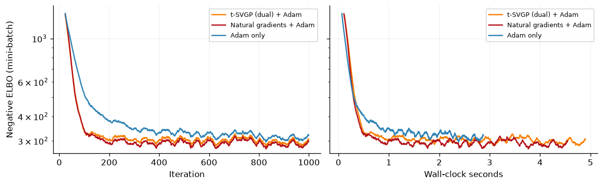
Both natural-gradient runs leave Adam behind per iteration, and both reach Adam’s thousand-iteration bound in a fraction of the wall-clock time Adam needed for it — the crossings are printed above.

What the timings do not show is a cheaper dual iteration. On this problem the two natural-gradient runs cost within a few percent of each other per iteration, with the dual one marginally the more expensive. The round trip the dual parameterisation avoids is \(\mathcal{O}(M^3)\) at \(M=50\), which is nothing next to the \(\mathcal{O}(BM^2)\) marginals at \(B=256\), so there is little to save here in the first place. (GPJax’s dual step also evaluates the objective once more per iteration than it strictly needs to, so that history[t] means the same thing in both branches — but under jit, which is how fit_natgrads always runs, XLA normally folds that repeat away, and nothing measured here separates the two effects.) Adam et al. report their gains at \(M=100\) with ten latent GPs and \(N=70{,}000\), where the constant they save is a much larger share of the total. Take the numbers above as a measurement of this configuration on this CPU, not as a refutation or a confirmation of theirs.

The two natural-gradient curves do not lie on top of each other, and the gap is far too large to be the \(10^{-3}\) that the beta_floor clip contributed a few cells ago. Up to that clip their E-steps are still the same iteration; what differs is that fit_natgrads interleaves an Adam step on the kernel hyperparameters and the inducing inputs, and the objective it differentiates for that step is dual_elbo in one run and elbo in the other. Those two have the same value and different hyperparameter gradients away from a converged E-step — and with \(\gamma\) ramping up from \(10^{-4}\), the E-step spends most of the first hundred iterations far from converged. From iteration 1 onwards the two runs are optimising the same model from different hyperparameters, and they never rejoin.

Which way does the divergence go? Here the dual run ends at the higher, that is worse, negative ELBO of the two; both final values are printed above. That is one seed, on a mini-batch bound, with the kernel hyperparameters and all fifty inducing inputs moving under a ramping \(\gamma\) — the two runs sit at different \(\boldsymbol{\theta}\) from iteration 1, so this is not a controlled comparison of the two M-step objectives and should not be read as one, in either direction. The controlled version — frozen inducing inputs, one kernel hyperparameter, matched E-steps — is the VEM run at the end of the notebook. What this figure does establish is that the choice of M-step objective changes the trajectory by tens of nats, which is why the rest of the notebook is about that choice.

Hyperparameter learning: dual_elbo versus elbo

Variational EM alternates an E-step, which maximises the ELBO over \(q\) at fixed \(\boldsymbol{\theta}\), with an M-step, which maximises it over \(\boldsymbol{\theta}\) at fixed \(q\). “Fixed \(q\)” is the ambiguous part. In natural coordinates the E-step returns \(\boldsymbol{\eta}^*_t = \boldsymbol{\eta}_0(\boldsymbol{\theta}_t) + \boldsymbol{\lambda}^*_t\), and there are two ways to hold that still:

\[\text{standard:}\quad l(\boldsymbol{\theta}) = \mathcal{L}\big(\underbrace{\boldsymbol{\eta}_0(\boldsymbol{\theta}_t) + \boldsymbol{\lambda}^*_t}_{\text{all frozen}},\ \boldsymbol{\theta}\big), \qquad\qquad \text{dual:}\quad \bar l(\boldsymbol{\theta}) = \mathcal{L}\big(\boldsymbol{\eta}_0(\boldsymbol{\theta}) + \boldsymbol{\lambda}^*_t,\ \boldsymbol{\theta}\big).\]

elbo computes the first, because a VariationalGaussian stores \((\mathbf{m},\mathbf{L})\) and those are what stay fixed. dual_elbo computes the second, because a DualVariationalGaussian stores the sites, and the prior half of \(q\) is rebuilt from \(\mathbf{K}_{zz}(\boldsymbol{\theta})\) every time the bound is evaluated. The intuition is that the sites encode what the data said, which is a property of the likelihood and should not be re-derived when the kernel moves, whereas the prior contribution to \(q\) should move with the kernel.

That is also why nothing derived from \(\boldsymbol{\theta}\) may be cached on the family. Caching \((\mathbf{m},\mathbf{S})\) would turn dual_elbo back into elbo under differentiation while leaving every printed value identical — a silent bug of the worst kind.

Here is what is actually guaranteed, which is less than the headline suggests:

claim	status
\(\bar l\) is a valid lower bound on \(\log p_{\boldsymbol{\theta}}(\mathbf{y})\) everywhere	proven — it is the ELBO at a legitimate Gaussian \(q\)
\(\bar l(\boldsymbol{\theta}_t) = l(\boldsymbol{\theta}_t)\)	proven, exactly, at a converged E-step
\(\nabla_{\boldsymbol{\theta}}\bar l(\boldsymbol{\theta}_t) = \nabla_{\boldsymbol{\theta}}l(\boldsymbol{\theta}_t)\)	proven, same condition, by the envelope theorem
\(\bar l(\boldsymbol{\theta}) \ge l(\boldsymbol{\theta})\) for all \(\boldsymbol{\theta}\)	proven only when the sites are genuinely \(\boldsymbol{\theta}\)-free — a conjugate likelihood with its exact sites and \(\mathbf{Z} = \mathbf{X}\), which is the regime of the second demo below
\(\bar l\) is a local upper bound on \(l\)	proven in the conjugate case; the paper writes “we can’t show this in the non-conjugate setting”
faster EM convergence when non-conjugate	empirical only — “exact theoretical reasons behind the speed-ups are currently unknown to us”

The honest headline: the two bounds agree in value and gradient at a converged E-step, and the dual M-step objective is less sensitive to \(\boldsymbol{\theta}_{\text{old}}\), which permits larger M-steps. It is not a uniformly tighter bound in the general sparse case. Take the claims in order.

def kernel_gradient(variational, hyper, objective, dataset):
    """Gradient of `objective` with respect to the unconstrained kernel parameters."""

    def loss(hyper):
        return objective(paramax.unwrap(eqx.combine(variational, hyper)), dataset)

    gradient = eqx.filter_grad(loss)(hyper)
    leaves = jtu.tree_leaves(gradient.model.prior.kernel)
    return jnp.concatenate([jnp.atleast_1d(jnp.ravel(leaf)) for leaf in leaves])


print("E-steps   max |grad dual_elbo - grad elbo|   |grad dual_elbo|")
for num_e_steps in [0, 1, 3, 6, 20, 60]:
    site_partition, site_hyper = partition_variational(logit_dual)
    moment_partition, moment_hyper = partition_variational(logit_moments)
    for _ in range(num_e_steps):
        site_partition, _ = natural_gradient_step(
            site_partition, site_hyper, logit_data, negative_dual_elbo, 0.8
        )
        moment_partition, _ = natural_gradient_step(
            moment_partition, moment_hyper, logit_data, negative_elbo, 0.8
        )
    site_gradient = kernel_gradient(
        site_partition, site_hyper, negative_dual_elbo, logit_data
    )
    moment_gradient = kernel_gradient(
        moment_partition, moment_hyper, negative_elbo, logit_data
    )
    print(
        f"{num_e_steps:7d}   "
        f"{float(jnp.max(jnp.abs(site_gradient - moment_gradient))):24.3e}   "
        f"{float(jnp.max(jnp.abs(site_gradient))):.3e}"
    )

E-steps   max |grad dual_elbo - grad elbo|   |grad dual_elbo|
      0                  3.898e+01   3.947e+01
      1                  1.596e+00   5.733e+00
      3                  7.155e-03   5.415e+00
      6                  5.909e-04   5.436e+00
     20                  6.492e-10   5.437e+00
     60                  3.730e-14   5.437e+00

The gradients converge onto each other as the E-step converges, which is the envelope theorem doing its work: at a stationary \(q\) the implicit dependence of the prior half of \(\boldsymbol{\eta}\) on \(\boldsymbol{\theta}\) contributes nothing. Away from stationarity the difference is not a rounding effect but a different vector: at the shared initialisation the two gradients disagree by as much as the whole magnitude of either one.

So the two M-step objectives can only differ when the E-step is incomplete, which in practice is always: nobody runs an E-step to convergence between Adam steps. The question is whether the difference helps. Freeze the sites at their \(\boldsymbol{\theta}_t\) values and slide the lengthscale.

log_offsets = jnp.linspace(-1.2, 0.6, 61)
frozen_sites, frozen_moments = exact_sites(
    regression_lengthscale, regression_inducing, regression_data
)


def bound_slice(inducing_inputs, dataset, sites, moments, offsets):
    """`dual_elbo` and `elbo` along a log-lengthscale slice, at frozen q."""
    dual_values, moment_values = [], []
    for offset in offsets:
        lengthscale = regression_lengthscale * jnp.exp(offset)
        dual_values.append(
            dual_elbo(
                paramax.unwrap(site_family(lengthscale, inducing_inputs, sites)),
                dataset,
            )
        )
        moment_values.append(
            elbo(
                paramax.unwrap(moment_family(lengthscale, inducing_inputs, moments)),
                dataset,
            )
        )
    return jnp.array(dual_values), jnp.array(moment_values)


dual_slice, moment_slice = bound_slice(
    regression_inducing, regression_data, frozen_sites, frozen_moments, log_offsets
)

# The slice is not symmetric about theta_t, so print both of its ends.
reference_index = int(jnp.argmin(jnp.abs(log_offsets)))
inducing_spacing = float(regression_inducing[1, 0] - regression_inducing[0, 0])
shortest_lengthscale = float(regression_lengthscale * jnp.exp(log_offsets[0]))
print("delta log-l        dual_elbo          elbo")
for label, index in [
    ("left edge ", 0),
    ("at theta_t", reference_index),
    ("right edge", len(log_offsets) - 1),
]:
    print(
        f"{label} {float(log_offsets[index]):+5.2f}  {float(dual_slice[index]):12.2f}  "
        f"{float(moment_slice[index]):14.2f}"
    )
print(
    f"inducing spacing {inducing_spacing:.3f}, shortest lengthscale on the slice "
    f"{shortest_lengthscale:.3f}"
)

fig, axes = plt.subplots(ncols=2, figsize=(10, 3.0))
axes[0].plot(log_offsets, dual_slice, color=cols[2], label=r"$\bar l$ (dual_elbo)")
axes[0].plot(log_offsets, moment_slice, color=cols[1], label=r"$l$ (elbo)")
axes[0].axvline(0.0, color="black", linestyle="--", linewidth=1)
axes[0].set(
    xlabel=r"$\Delta\log\ell$ from $\theta_t$",
    ylabel="Bound (nats)",
    ylim=(float(dual_slice.min()) - 40.0, float(dual_slice.max()) + 10.0),
    title=f"Sparse, $M = {num_inducing}$",
)
clean_legend(axes[0])

for inducing_count, colour in [(5, cols[0]), (10, cols[3]), (20, cols[2])]:
    sparse_inducing = jnp.linspace(-3.0, 3.0, inducing_count).reshape(-1, 1)
    sparse_sites, sparse_moments = exact_sites(
        regression_lengthscale, sparse_inducing, regression_data
    )
    sparse_dual, sparse_moment = bound_slice(
        sparse_inducing, regression_data, sparse_sites, sparse_moments, log_offsets
    )
    gap = sparse_dual - sparse_moment
    axes[1].plot(log_offsets, gap, color=colour, label=f"$M = {inducing_count}$")
    print(
        f"M = {inducing_count:2d}: smallest gap {float(gap.min()):+.4e} nats at "
        f"delta log-lengthscale {float(log_offsets[jnp.argmin(gap)]):+.3f}"
    )
axes[1].axhline(0.0, color="black", linestyle="--", linewidth=1)
axes[1].set(
    xlabel=r"$\Delta\log\ell$ from $\theta_t$",
    ylabel=r"$\bar l - l$ (nats)",
    yscale="symlog",
    title="Dominance is not uniform when sparse",
)
clean_legend(axes[1])

delta log-l        dual_elbo          elbo
left edge  -1.20       -315.72         -321.96
at theta_t -0.00        -82.66          -82.66
right edge +0.60        -76.66        -5430.16
inducing spacing 0.316, shortest lengthscale on the slice 0.151
M =  5: smallest gap -2.6678e-01 nats at delta log-lengthscale +0.600
M = 10: smallest gap -3.2758e-01 nats at delta log-lengthscale -0.960
M = 20: smallest gap +0.0000e+00 nats at delta log-lengthscale -0.000

<Axes: title={'center': 'Dominance is not uniform when sparse'}, xlabel='$\\Delta\\log\\ell$ from $\\theta_t$', ylabel='$\\bar l - l$ (nats)'>

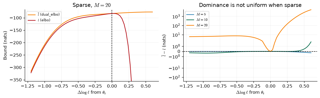
The left panel is the shape the paper’s Fig. 2 is about, and the honest reading of it is asymmetric. Both bounds pass through the same point at \(\boldsymbol{\theta}_t\) — that is the value-equality row of the table, and it holds to \(7\times10^{-14}\) here, which is the \(M=20\) minimum printed above.

To the right, at longer lengthscales, \(l\) falls off a cliff — the printed right-edge values put it more than \(10^{5}\) nats below \(\bar l\) — because a \(q\) whose covariance was chosen for one kernel is a bad approximation under another, but \(\bar l\) has barely moved, since only the data-dependent half of it was frozen. To the left the two collapse together instead, within a few nats of each other and both a couple of hundred nats below their value at \(\boldsymbol{\theta}_t\). That is not the freezing failing but the sparse approximation itself: by the left-hand edge the lengthscale has dropped below half the inducing spacing — both are printed above — so \(\mathbf{Q}_{ff}\) is a poor stand-in for \(\mathbf{K}_{ff}\) and no choice of frozen \(q\) rescues it. Since the M-step travels rightwards out of a too-short lengthscale, the asymmetry is the useful half: in the direction of travel an M-step on \(\bar l\) can go much further before the bound it is climbing stops being informative.

The right panel is the caveat. At \(M=20\) the dual bound dominates everywhere we looked, up to float64 noise at the crossing point — the printed \(M=20\) minimum is negative at the \(10^{-14}\) level and sits at \(\Delta\log\ell = 0\), which is the value-equality point itself. At \(M=5\) and \(M=10\) the gap dips below zero for real — the minima are printed above — and the guarantee does not hold. The reason is precise: with \(\mathbf{Z}\neq\mathbf{X}\) the flanked sites \(\boldsymbol{\lambda}_1^\star = \mathbf{K}_{zz}^{-1}\mathbf{K}_{zx}(\mathbf{y}-\boldsymbol{\mu}_x)/\sigma^2\) still depend on \(\boldsymbol{\theta}\) through \(\mathbf{K}_{zx}\), so freezing them at \(\boldsymbol{\theta}_t\) makes \(\boldsymbol{\eta}_0(\boldsymbol{\theta})+\boldsymbol{\lambda}^*_t\) sub-optimal elsewhere and the proof’s hypothesis fails. Remove the sparsity and the hypothesis holds exactly.

# Z = X: the sites collapse to (y - mu) / sigma^2 and I / sigma^2, free of theta.
dense_count = 40
dense_inputs = regression_inputs[:dense_count]
dense_outputs = regression_outputs[:dense_count]
dense_data = gpx.Dataset(X=dense_inputs, y=dense_outputs)

dense_sites, dense_moments = exact_sites(
    regression_lengthscale, dense_inputs, dense_data
)
dense_prior = paramax.unwrap(
    site_family(regression_lengthscale, dense_inputs)
).model.prior
dense_gram = dense_prior.kernel.gram(
    dense_inputs
).as_matrix() + regression_jitter * jnp.eye(dense_count)
dense_centred = dense_outputs - dense_prior.mean_function(dense_inputs)

exact_dual_vector = dense_centred / observation_variance
exact_dual_matrix = jnp.eye(dense_count) / observation_variance
flanked_error = jnp.max(jnp.abs(dense_gram @ (dense_sites[0] - exact_dual_vector)))
flanked_scale = jnp.max(jnp.abs(dense_gram @ exact_dual_vector))

print(f"cond(K_zz) at Z = X                : {jnp.linalg.cond(dense_gram):.3e}")
print(
    "max |Lambda_2 - I / sigma^2|       : "
    f"{jnp.max(jnp.abs(dense_sites[1] - exact_dual_matrix)):.3e}   (never test this)"
)
print(
    "relative error of K_zz lambda_1    : "
    f"{float(flanked_error / flanked_scale):.3e}   (test this instead)"
)

dense_offsets = jnp.linspace(-0.6, 0.6, 41)
dense_dual_slice, dense_moment_slice = bound_slice(
    dense_inputs, dense_data, dense_sites, dense_moments, dense_offsets
)

fig, ax = plt.subplots(figsize=(5.5, 3.2))
ax.plot(dense_offsets, dense_dual_slice, color=cols[2], label=r"$\bar l$ (dual_elbo)")
ax.plot(dense_offsets, dense_moment_slice, color=cols[1], label=r"$l$ (elbo)")
ax.axvline(0.0, color="black", linestyle="--", linewidth=1)
ax.set(
    xlabel=r"$\Delta\log\ell$ from $\theta_t$",
    ylabel="Bound (nats)",
    yscale="symlog",
    title=r"$Z = X$: dominance holds",
)
clean_legend(ax)

dense_gap = dense_dual_slice - dense_moment_slice
print(f"smallest gap over the slice        : {float(dense_gap.min()):+.3e} nats")
print(f"largest gap over the slice         : {float(dense_gap.max()):+.3e} nats")

cond(K_zz) at Z = X                : 1.042e+09
max |Lambda_2 - I / sigma^2|       : 8.954e+00   (never test this)
relative error of K_zz lambda_1    : 2.433e-07   (test this instead)
smallest gap over the slice        : +5.684e-14 nats
largest gap over the slice         : +8.554e+03 nats

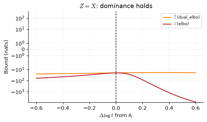
With no sparsity gap the dual bound dominates over the whole slice, by several orders of magnitude, and stays finite where \(l\) collapses through decades on a symlog axis. The smallest gap is float64 noise at the crossing point, not a violation.

The two diagnostic lines above the plot are the conditioning story promised earlier, and they are worth reading together. At \(\mathbf{Z}=\mathbf{X}\) the analytic answer for the stored matrix is \(\boldsymbol{\Lambda}_2 = \mathbf{I}/\sigma^2\), and the computed one is wrong by several units entrywise, because forming it needs \(\mathbf{K}_{zz}^{-1}\) twice at a condition number near \(10^9\). Yet \(\mathbf{K}_{zz}\boldsymbol{\lambda}_1\) — the flanked quantity that everything downstream actually consumes — is right to nine digits, and the bound plotted above is smooth. The error lives in the near-null space of \(\mathbf{K}_{zz}\) and is annihilated on the way back out. That is a measurement in one configuration and not a theorem, which is exactly why the rule is to test \(\mathbf{R}\), the moments or the predictions, and never \(\boldsymbol{\Lambda}_2\) itself.

The M-step in a loop

Bound slices are static. The claim that actually matters is that a real VEM loop gets further with dual_elbo as its M-step objective, and that one is empirical: the paper says as much. So we run it. Both branches share the same E-step — the same iteration, up to the beta_floor clip located earlier — and differ only in what the M-step differentiates. The inducing inputs are frozen so that only the kernel moves, and the lengthscale starts five times too short.

expectation_steps = 20
maximisation_steps = 5
vem_rounds = 40
vem_rate = 0.5
vem_optimiser = ox.adam(5e-2)
initial_lengthscale = 0.25


def freeze_inducing(model):
    """Hold the inducing inputs still, so the M-step moves only the kernel."""
    return eqx.tree_at(
        lambda tree: tree.inducing_inputs,
        model,
        paramax.non_trainable(model.inducing_inputs),
    )


def vem_joint_model(lengthscale):
    return (
        gpx.gps.Prior(
            mean_function=gpx.mean_functions.Zero(),
            kernel=jk.RBF(active_dims=[0, 1], lengthscale=lengthscale),
            jitter=banana_jitter,
        )
        * gpx.likelihoods.Bernoulli()
    )


vem_gram = paramax.unwrap(vem_joint_model(initial_lengthscale)).prior.kernel.gram(
    banana_inducing
).as_matrix() + banana_jitter * jnp.eye(num_banana_inducing)

vem_dual = freeze_inducing(
    DualVariationalGaussian(
        model=vem_joint_model(initial_lengthscale),
        inducing_inputs=banana_inducing,
    )
)
vem_moments = freeze_inducing(
    VariationalGaussian(
        model=vem_joint_model(initial_lengthscale),
        inducing_inputs=banana_inducing,
        variational_mean=jnp.zeros((num_banana_inducing, 1)),
        variational_root_covariance=jnp.linalg.cholesky(vem_gram),
    )
)


def run_vem(model, objective):
    """Alternate `expectation_steps` E-steps with `maximisation_steps` M-steps."""
    variational, hyper = partition_variational(model)
    opt_state = vem_optimiser.init(eqx.filter(hyper, eqx.is_array))

    @eqx.filter_jit
    def expectation_step(variational, hyper):
        def body(carry, _):
            updated, _ = natural_gradient_step(
                carry, hyper, banana_train, objective, vem_rate
            )
            return updated, None

        return jax.lax.scan(body, variational, None, length=expectation_steps)[0]

    @eqx.filter_jit
    def maximisation_step(variational, hyper, opt_state):
        def hyper_loss(hyper):
            return objective(
                paramax.unwrap(eqx.combine(variational, hyper)), banana_train
            )

        def body(carry, _):
            hyper, opt_state = carry
            loss, gradient = eqx.filter_value_and_grad(hyper_loss)(hyper)
            updates, opt_state = vem_optimiser.update(
                gradient, opt_state, eqx.filter(hyper, eqx.is_array)
            )
            return (eqx.apply_updates(hyper, updates), opt_state), loss

        (hyper, opt_state), losses = jax.lax.scan(
            body, (hyper, opt_state), None, length=maximisation_steps
        )
        return hyper, opt_state, losses[-1]

    lengthscales, bounds = [], []
    for _ in range(vem_rounds):
        variational = expectation_step(variational, hyper)
        hyper, opt_state, loss = maximisation_step(variational, hyper, opt_state)
        combined = paramax.unwrap(eqx.combine(variational, hyper))
        lengthscales.append(float(combined.model.prior.kernel.lengthscale))
        bounds.append(float(loss))
    return eqx.combine(variational, hyper), jnp.array(lengthscales), jnp.array(bounds)


dual_vem_model, dual_lengthscales, dual_bounds = run_vem(vem_dual, negative_dual_elbo)
moment_vem_model, moment_lengthscales, moment_bounds = run_vem(
    vem_moments, negative_elbo
)

fig, axes = plt.subplots(ncols=2, figsize=(10, 3.0))
rounds = jnp.arange(1, vem_rounds + 1)
for name, lengthscales, colour in [
    ("M-step on dual_elbo", dual_lengthscales, cols[2]),
    ("M-step on elbo", moment_lengthscales, cols[1]),
]:
    axes[0].plot(rounds, lengthscales, color=colour, label=name)
axes[0].set(xlabel="VEM round", ylabel=r"Lengthscale $\ell$")
clean_legend(axes[0])

# The two bound traces are visually identical at this scale, so plot their difference:
# positive means the dual M-step is the further down the negative ELBO of the two.
bound_lead = moment_bounds - dual_bounds
axes[1].plot(rounds, bound_lead, color=cols[2])
axes[1].axhline(0.0, color="black", linestyle="--", linewidth=1)
axes[1].set(
    xlabel="VEM round",
    ylabel="Bound lead to dual_elbo (nats)",
    title="Lead of the dual M-step over the standard one",
)


def test_metrics(model):
    """Held-out accuracy and negative log predictive density."""
    unwrapped = paramax.unwrap(model)
    probability = unwrapped.model.likelihood(unwrapped(test_inputs_2d)).mean
    labels = test_labels.ravel()
    log_density = jnp.mean(
        labels * jnp.log(probability) + (1.0 - labels) * jnp.log1p(-probability)
    )
    return float(jnp.mean((probability > 0.5) == (labels > 0.5))), float(-log_density)


for name, model, lengthscales, bounds in [
    ("dual_elbo", dual_vem_model, dual_lengthscales, dual_bounds),
    ("elbo     ", moment_vem_model, moment_lengthscales, moment_bounds),
]:
    accuracy, nlpd = test_metrics(model)
    print(
        f"M-step on {name}: lengthscale {float(lengthscales[-1]):.4f}, "
        f"negative ELBO {float(bounds[-1]):8.3f}, "
        f"test accuracy {accuracy:.4f}, test NLPD {nlpd:.4f}"
    )
print(
    f"bound lead to dual_elbo over {vem_rounds} rounds: "
    f"smallest {float(bound_lead.min()):+.3f}, largest {float(bound_lead.max()):+.3f}, "
    f"final {float(bound_lead[-1]):+.3f} nats"
)
# Sentinel above every attainable round, so "never" stays distinguishable.
never_positive = vem_rounds + 1
crossing_round = int(jnp.min(jnp.where(bound_lead > 0.0, rounds, never_positive)))
if crossing_round == never_positive:
    print("the dual M-step never takes the lead")
else:
    print(
        f"first round with a positive lead: {crossing_round}; smallest lead from "
        f"there on: {float(bound_lead[crossing_round - 1 :].min()):+.3f} nats"
    )

M-step on dual_elbo: lengthscale 1.4127, negative ELBO  295.759, test accuracy 0.9300, test NLPD 0.1626
M-step on elbo     : lengthscale 1.3636, negative ELBO  296.601, test accuracy 0.9300, test NLPD 0.1625
bound lead to dual_elbo over 40 rounds: smallest -1.149, largest +1.266, final +0.842 nats
first round with a positive lead: 1; smallest lead from there on: -1.149 nats

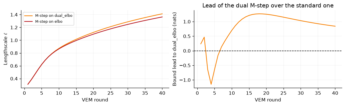
The two lengthscale traces sit on top of each other for the first several rounds and then separate, with the dual branch ending the longer of the two; both final values are printed above. The right panel is the difference of the two bounds rather than the two bounds themselves, and that is deliberate: on a negative ELBO of around 294 a lead of a nat is invisible, so the traces would be indistinguishable and the sign of the difference — the whole question — unreadable.

The sign changes. Over the opening rounds the dual branch is behind, by up to a few nats, while both are still far from the optimum and moving fast; it takes the lead at the printed crossing round and does not give it back, peaking below a nat and ending at the printed final value. So the honest reading is not “the dual M-step is uniformly ahead”. It is that the two branches take different routes to the same place: after forty rounds the dual one has the longer lengthscale and the marginally better bound, and their held-out NLPDs agree to three decimal places. That is consistent with the theory, which promises equality at convergence and says nothing about the rate — “exact theoretical reasons behind the speed-ups are currently unknown to us”.

It is also a soft result on a two-dimensional problem with one kernel hyperparameter and fifty fixed inducing points. The regime the paper reports gains in — many latent GPs, large \(N\), mini-batched, hyperparameters far from their optimum — is not this one. Read the demo as a mechanism check rather than as a benchmark, and if you want the mechanism in one sentence: at an incomplete E-step the two objectives have different hyperparameter gradients, and the dual one is the gradient of a function that still knows the prior depends on \(\boldsymbol{\theta}\).

Caveats

• One latent process. Everything above assumes \(L=1\). The site structure across multiple latent GPs is block diagonal only when the variational family is itself latent diagonal, and the tied projection has to be re-derived rather than reused for a multi-output model. DualVariationalGaussian targets the scalar case.

• \(\beta_i \ge 0\) needs a log-concave likelihood — as computed, not as written. Student-\(t\) and some heteroscedastic likelihoods are not log-concave at all, and for those the target can push \(\boldsymbol{\Lambda}_2\) out of the PSD cone. Less obviously, GPJax’s Bernoulli joins them in the far tails: inv_probit clips its output into \([10^{-3},\,1-10^{-3}]\), which flattens \(\log p\) and makes its second derivative positive for \(f \lesssim -2.44\), so a confidently mislabelled point yields \(\beta_i < 0\). The beta_floor keyword (default \(10^{-8}\)) clips \(\boldsymbol{\beta}\) from below and keeps the step inside the cone. It is not a no-op for Bernoulli — it is what breaks the \(\rho=\gamma\) identity on the banana demo above, by \(\sim\!10^{-3}\) in \((\mathbf{m},\mathbf{S})\). Note that it clips \(\boldsymbol{\beta}\), never \(\boldsymbol{\Lambda}_2\): the update stays affine, so it stays jit- and scan-safe.

• \(\rho \in (0,1]\). The convex-combination guarantee stops at \(1\), and beyond it the step extrapolates past a target that is only locally valid. fit_natgrads rejects a larger constant rate for this family at call time.

• Flanked storage squares \(\operatorname{cond}(\mathbf{K}_{zz})\). Benign in everything measured here at the level of \(\mathbf{R}\), the moments and the bound, and visibly not benign entrywise in \(\boldsymbol{\Lambda}_2\). Never write a test against \(\boldsymbol{\Lambda}_2\) directly.

• The E-step is not a free lunch. Wherever the computed \(\beta_i\) stay non-negative it is the same iteration as the natural gradient step on \((\mathbf{m},\mathbf{L})\), and where they do not the difference is the clip above, not a better search direction. Whatever the dual parameterisation buys is either wall-clock per iteration or M-step behaviour; none of it is a better \(q\) at the same \(\boldsymbol{\theta}\).

For the geometry the E-step is built on — the Fisher identity, mirror descent, the negative-definite cone and the step-size backoff — see the natural gradients notebook.

System configuration

%reload_ext watermark
%watermark -n -u -v -iv -w -a 'Thomas Pinder'

Author: Thomas Pinder

Last updated: Fri, 07 Aug 2026

Python implementation: CPython
Python version       : 3.11.15
IPython version      : 9.15.0

equinox   : 0.13.8
gpjax     : 0.18.0
jax       : 0.10.2
jaxtyping : 0.3.11
matplotlib: 3.11.1
optax     : 0.2.8
paramax   : 0.0.5

Watermark: 2.6.0