Natural Gradients#
Download this notebook: natgrads.ipynb
Variational inference in a sparse Gaussian process asks us to optimise a probability distribution \(q(\mathbf{u})\), not a point in \(\mathbb{R}^P\). Gradient descent does not know that: it moves the storage coordinates of \(q\) — a mean vector and a Cholesky factor — as though they lived in flat Euclidean space, and so the step it takes depends on how we happened to write the distribution down. The natural gradient repairs this by measuring distance between distributions with the Fisher information metric, which makes the update invariant to the parameterisation.
This notebook implements the recipe of
Salimbeni et al. [2018], which is what
gpjax.fit_natgrads runs. The remarkable practical point is that for a Gaussian
process the natural gradient costs no Fisher matrix at all: the Fisher information
turns out to be the Jacobian \(\partial\boldsymbol{\eta}/\partial\boldsymbol{\theta}\)
between two standard coordinate systems, so the natural gradient with respect to one
of them is the plain gradient with respect to the other.
The route is:
write \(q(\mathbf{u})\) in exponential-family form and name its two canonical coordinate systems, the natural parameters \(\boldsymbol{\theta}\) and the expectation parameters \(\boldsymbol{\eta}\);
show that the Fisher matrix is \(\partial\boldsymbol{\eta}/\partial\boldsymbol{\theta}\), and check it numerically;
read the step as mirror descent, which explains why \(\gamma \le 1\) is special;
demo (i) — a conjugate 1D regression where a single \(\gamma=1\) step lands on the exact variational optimum (which, at the \(M=20\) inducing points used there, is indistinguishable from the full GP posterior), while Adam is still crawling after two thousand;
demo (ii) — a mini-batched Bernoulli classification benchmark, comparing natural gradients + Adam against Adam alone, per iteration and per second;
the failure mode: what a large \(\gamma\) does, and how the built-in step-size backoff behaves.
If you have not met sparse variational GPs before, read the stochastic sparse GP notebook first — everything below assumes the SVGP evidence lower bound.
# Enable Float64 for more stable matrix inversions.
import time

import equinox as eqx
import jax
from jax import config
import jax.numpy as jnp
import jax.random as jr
from jaxtyping import install_import_hook
import matplotlib as mpl
import matplotlib.pyplot as plt
import optax as ox
import paramax
from utils import clean_legend, use_mpl_style

config.update("jax_enable_x64", True)


with install_import_hook("gpjax", "beartype.beartype"):
    import gpjax as gpx
    import gpjax.kernels as jk
    from gpjax.natural_gradients import (
        expectation_from_moments,
        moments_from_expectation,
        moments_from_natural,
        natural_from_moments,
        natural_gradient_step,
        partition_variational,
    )
    from gpjax.parameters import LowerTriangular, Real

key = jr.key(123)

# set the default style for plotting
use_mpl_style()
cols = mpl.rcParams["axes.prop_cycle"].by_key()["color"]


def negative_elbo(model, data):
    """The loss every fit below minimises: GPJax optimisers descend, so negate."""
    return -gpx.objectives.elbo(model, data)
The exponential-family view#
The variational distribution over the inducing outputs is \(q(\mathbf{u}) = \mathcal{N}(\mathbf{m}, \mathbf{S})\) with \(\mathbf{m}\) of shape \(M\times 1\) and \(\mathbf{S}\) of shape \(M \times M\). Written as an exponential family,
with sufficient statistics \(\mathbf{t}(\mathbf{u}) = [\,\mathbf{u},\ \operatorname{vec}(\mathbf{u}\mathbf{u}^\top)\,]\). Matching terms gives the natural parameters
so that \(\boldsymbol{\theta}^\top\mathbf{t}(\mathbf{u}) = \mathbf{u}^\top\boldsymbol{\theta}_1 + \mathbf{u}^\top\boldsymbol{\Theta}_2\mathbf{u}\). The expectation parameters are the mean of the sufficient statistics, \(\boldsymbol{\eta} = \mathbb{E}_q[\mathbf{t}(\mathbf{u})]\):
The log normaliser is
and differentiating it recovers the expectation parameters, \(\nabla_{\boldsymbol{\theta}}A(\boldsymbol{\theta}) = \boldsymbol{\eta}\) — the standard duality between the two coordinate systems.
There is a third coordinate system in play, the one GPJax actually stores:
\(\boldsymbol{\xi} = (\mathbf{m}, \mathbf{L})\) with \(\mathbf{S} = \mathbf{L}\mathbf{L}^\top\)
and \(\mathbf{L}\) lower triangular with a positive diagonal. That choice keeps
\(\mathbf{S}\) positive definite under any unconstrained optimiser, but it is a
storage convention, not a geometry. gpjax.natural_gradients exposes the four maps
that connect the three systems — expectation_from_moments,
natural_from_moments, moments_from_expectation and moments_from_natural — each
built from Cholesky factors and triangular solves, with no explicit matrix inverse
anywhere.
The Fisher information is the Jacobian \(\partial\boldsymbol{\eta}/\partial\boldsymbol{\theta}\)#
Differentiating \(\log q\) twice with respect to \(\boldsymbol{\theta}\) kills the sufficient statistics and leaves only the log normaliser, so
The Fisher information of an exponential family is simultaneously the Hessian of its log normaliser, the Jacobian from natural to expectation parameters, and the covariance of its sufficient statistics. The middle equality is the one that pays. Let \(\ell\) be a loss (for us, the negative ELBO). The chain rule in row-gradient form reads \(\partial\ell/\partial\boldsymbol{\theta} = (\partial\ell/\partial\boldsymbol{\eta})(\partial\boldsymbol{\eta}/\partial\boldsymbol{\theta})\); transposing to column gradients and using the self-adjointness of \(\mathbf{F} = \mathrm{D}\boldsymbol{\eta}\) (it is a Hessian) gives \((\partial\ell/\partial\boldsymbol{\theta}) = \mathbf{F}(\partial\ell/\partial\boldsymbol{\eta})\), so that
The gradient with respect to the expectation parameters is the natural gradient with respect to the natural parameters. No Fisher matrix is built, and no linear system is solved. The update is
with \(\gamma\) the step size, called natgrad_lr in GPJax.
One technical caveat before we check this numerically. The statistic \(\operatorname{vec}(\mathbf{u}\mathbf{u}^\top)\) has \(M^2\) entries, but \(q\) depends on \(\boldsymbol{\Theta}_2\) only through its symmetric part, so in those redundant coordinates \(\mathbf{F}\) is singular and \(\mathbf{F}^{-1}\) is not defined. The fix is to work on the space of symmetric matrices with the trace inner product \(\langle \mathbf{A},\mathbf{B}\rangle = \operatorname{tr}(\mathbf{A}\mathbf{B})\); concretely, flatten a symmetric matrix by stacking its lower triangle with the strictly off-diagonal entries scaled by \(\sqrt{2}\). In those coordinates the Euclidean gradient is the correct gradient and \(\mathbf{F}\) is symmetric positive definite. The production step never forms \(\mathbf{F}\) and so never needs any of this; we need it only to verify the identity.
# A small non-conjugate model (Bernoulli likelihood, M = 3) on which to check
# F^{-1} dl/dtheta == dl/deta directly.
key, input_key, label_key, mean_key, root_key = jr.split(key, 5)

check_inputs = jr.uniform(input_key, (30, 1), minval=-2.0, maxval=2.0)
check_labels = (
    jr.uniform(label_key, (30, 1)) < jax.nn.sigmoid(2.0 * check_inputs)
).astype(jnp.float64)
check_data = gpx.Dataset(X=check_inputs, y=check_labels)

check_model = (
    gpx.gps.Prior(mean_function=gpx.mean_functions.Zero(), kernel=jk.RBF())
    * gpx.likelihoods.Bernoulli()
)

num_check_inducing = 3
check_mean = 0.5 * jr.normal(mean_key, (num_check_inducing, 1))
check_factor = 0.5 * jr.normal(root_key, (num_check_inducing, num_check_inducing))
check_root = jnp.linalg.cholesky(
    check_factor @ check_factor.T + jnp.eye(num_check_inducing)
)
check_family = gpx.variational_families.VariationalGaussian(
    model=check_model,
    inducing_inputs=jnp.linspace(-2.0, 2.0, num_check_inducing).reshape(-1, 1),
    variational_mean=check_mean,
    variational_root_covariance=check_root,
)


def symmetric_to_vector(matrix):
    """Flatten a symmetric matrix isometrically: lower triangle, sqrt(2) off-diag."""
    size = matrix.shape[0]
    scale = jnp.where(jnp.eye(size, dtype=bool), 1.0, jnp.sqrt(2.0))
    rows, columns = jnp.tril_indices(size)
    return (matrix * scale)[rows, columns]


def vector_to_symmetric(vector, size):
    """Invert `symmetric_to_vector`."""
    rows, columns = jnp.tril_indices(size)
    lower = jnp.zeros((size, size)).at[rows, columns].set(vector)
    diagonal = jnp.diag(jnp.diag(lower))
    strictly_lower = (lower - diagonal) / jnp.sqrt(2.0)
    return diagonal + strictly_lower + strictly_lower.T


def pack(vector_part, matrix_part):
    return jnp.concatenate([vector_part.ravel(), symmetric_to_vector(matrix_part)])


def unpack(flat, size):
    return flat[:size].reshape(-1, 1), vector_to_symmetric(flat[size:], size)


def loss_at_moments(variational_mean, variational_root_covariance):
    trial = eqx.tree_at(
        lambda family: (family.variational_mean, family.variational_root_covariance),
        check_family,
        (Real(variational_mean), LowerTriangular(variational_root_covariance)),
    )
    return negative_elbo(paramax.unwrap(trial), check_data)


def loss_of_natural(flat):
    """The loss as a function of the flattened natural parameters."""
    return loss_at_moments(*moments_from_natural(*unpack(flat, num_check_inducing)))


def loss_of_expectation(flat):
    """The loss as a function of the flattened expectation parameters."""
    return loss_at_moments(*moments_from_expectation(*unpack(flat, num_check_inducing)))


def expectation_of_natural(flat):
    """The map whose Jacobian is the Fisher information."""
    moments = moments_from_natural(*unpack(flat, num_check_inducing))
    return pack(*expectation_from_moments(*moments))


flat_natural = pack(*natural_from_moments(check_mean, check_root))
flat_expectation = pack(*expectation_from_moments(check_mean, check_root))

fisher = jax.jacfwd(expectation_of_natural)(flat_natural)
natural_gradient = jnp.linalg.solve(fisher, jax.grad(loss_of_natural)(flat_natural))
expectation_gradient = jax.grad(loss_of_expectation)(flat_expectation)

print(f"asymmetry of F                    : {jnp.max(jnp.abs(fisher - fisher.T)):.3e}")
print(f"smallest eigenvalue of F          : {jnp.min(jnp.linalg.eigvalsh(fisher)):.4f}")
print(
    "max |F^-1 dl/dtheta - dl/deta|    : "
    f"{jnp.max(jnp.abs(natural_gradient - expectation_gradient)):.3e}"
)
asymmetry of F                    : 8.882e-16
smallest eigenvalue of F          : 0.6691
max |F^-1 dl/dtheta - dl/deta|    : 3.109e-15
\(\mathbf{F}\) is symmetric and positive definite, and the natural gradient obtained by solving with it agrees with the plain gradient in expectation coordinates to machine precision. Note that the solve just performed lives in the \(\operatorname{vec}_s\) coordinates introduced above, of dimension \(P = M + \tfrac{1}{2}M(M+1)\) — nine at \(M=3\) — and not in the \(M + M^2\) coordinates, where \(\mathbf{F}\) is singular. Everything from here on uses the right-hand side of the identity, so that \(\mathcal{O}(P^3) = \mathcal{O}(M^6)\) Fisher solve never happens again.
Mirror descent#
There is a second reading of the same update that explains the role of the step size. Let \(\Psi = A^*\) be the convex conjugate of the log normaliser — the negative entropy of \(q\) — so that \(\boldsymbol{\theta} = \nabla\Psi(\boldsymbol{\eta})\). Mirror ascent on the ELBO \(\mathcal{L}\) with mirror map \(\Psi\) is
which is precisely the natural-gradient step. The mirror-descent view is the reason \(\gamma \le 1\) is not an arbitrary convention: as we will see in a moment, the step is then a convex combination in \(\boldsymbol{\theta}\)-space between where \(q\) is and where the current data want it to be. Going beyond \(\gamma = 1\) is an extrapolation, and extrapolation is what breaks.
Conjugate models: one step is enough#
Suppose the ELBO can be written, for some fixed \(\boldsymbol{\lambda}\) that does not depend on \(q\),
that is, \(\mathbb{E}_q[\log p(\mathbf{y},\mathbf{u})]\) is affine in \(\boldsymbol{\eta}\). This is exactly the conditionally-conjugate case: a Gaussian likelihood. Since \(\mathbb{H}[q] = -\mathbb{E}_q[\log h] - \boldsymbol{\theta}^\top\boldsymbol{\eta} + A(\boldsymbol{\theta})\) and \(\partial A/\partial\boldsymbol{\theta} = \boldsymbol{\eta}\), the two Jacobian terms cancel and \(\partial\mathbb{H}/\partial\boldsymbol{\eta} = -\boldsymbol{\theta}\). Therefore
and \(\gamma = 1\) gives \(\boldsymbol{\theta}_{\text{new}} = \boldsymbol{\lambda} = \boldsymbol{\theta}^\star\) in one step, from any starting point. This is Sato’s (2001) observation that natural-gradient ascent at unit step size is the classical variational fixed-point update; for the SVGP it recovers the Titsias [2009] optimum.
Let us watch it happen.
# Demo (i): 1D conjugate regression.
num_data = 200
noise_stddev = 0.3

key, input_key, noise_key = jr.split(key, 3)
regression_inputs = jr.uniform(input_key, (num_data, 1), minval=-3.0, maxval=3.0)
regression_signal = jnp.sin(2.0 * regression_inputs)
regression_outputs = regression_signal + noise_stddev * jr.normal(
    noise_key, regression_signal.shape
)
regression_data = gpx.Dataset(X=regression_inputs, y=regression_outputs)

num_inducing = 20
regression_inducing = jnp.linspace(-3.0, 3.0, num_inducing).reshape(-1, 1)
test_inputs = jnp.linspace(-3.2, 3.2, 300).reshape(-1, 1)
# A conjugate SVGP, deliberately initialised a long way from its optimum. The joint
# model is prior * likelihood; the variational family approximates its posterior.
regression_model = gpx.gps.Prior(
    mean_function=gpx.mean_functions.Constant(),
    kernel=jk.RBF(lengthscale=0.5),
    jitter=1e-8,
) * gpx.likelihoods.Gaussian(obs_stddev=noise_stddev)

key, bad_mean_key, bad_root_key = jr.split(key, 3)
bad_mean = jr.normal(bad_mean_key, (num_inducing, 1))
bad_factor = 0.3 * jr.normal(bad_root_key, (num_inducing, num_inducing))
bad_root = jnp.linalg.cholesky(bad_factor @ bad_factor.T + 0.5 * jnp.eye(num_inducing))

initial_family = gpx.variational_families.WhitenedVariationalGaussian(
    model=regression_model,
    inducing_inputs=regression_inducing,
    variational_mean=bad_mean,
    variational_root_covariance=bad_root,
)
We use the whitened family here, which reparameterises
\(\mathbf{u} = \boldsymbol{\mu}_z + \mathbf{L}_z\mathbf{v}\) with
\(\mathbf{L}_z\mathbf{L}_z^\top = \mathbf{K}_{zz}\) and puts a
\(\mathcal{N}(\mathbf{0},\mathbf{I})\) prior on \(\mathbf{v}\). The natural-gradient
machinery is untouched by this — \(q(\mathbf{v})\) belongs to the same exponential
family, and the whitening enters only through prior_kl and predict, which the
loss calls polymorphically. Numerically it helps a great deal, because
\(\mathbf{m}_w\) and \(\mathbf{S}_w\) are \(\mathcal{O}(1)\) regardless of the kernel
scale, and the conjugate optimum satisfies
\(\mathbf{S}_w^\star \preceq \mathbf{I}\).
For the whitened family the closed-form optimum is, with \(\mathbf{A}_w = \mathbf{K}_{xz}\mathbf{L}_z^{-\top}\) and \(\sigma^2\) the observation variance,
unwrapped_initial = paramax.unwrap(initial_family)
kernel = unwrapped_initial.model.prior.kernel
mean_function = unwrapped_initial.model.prior.mean_function

Kzz = kernel.gram(regression_inducing).as_matrix()
Kzz = Kzz + initial_family.model.prior.jitter * jnp.eye(num_inducing)
Lz = jnp.linalg.cholesky(Kzz)
Kzx = kernel.cross_covariance(regression_inducing, regression_inputs)
whitened_design = jax.scipy.linalg.solve_triangular(Lz, Kzx, lower=True).T

observation_variance = noise_stddev**2
whitened_precision = (
    jnp.eye(num_inducing) + whitened_design.T @ whitened_design / observation_variance
)
whitened_shift = (
    whitened_design.T
    @ (regression_outputs - mean_function(regression_inputs))
    / observation_variance
)
optimal_covariance = jnp.linalg.inv(whitened_precision)
optimal_mean = jnp.linalg.solve(whitened_precision, whitened_shift)

# The ELBO at the closed-form optimum, used below as the reference for both methods.
optimal_family = eqx.tree_at(
    lambda family: (family.variational_mean, family.variational_root_covariance),
    initial_family,
    (Real(optimal_mean), LowerTriangular(jnp.linalg.cholesky(optimal_covariance))),
)
reference_elbo = float(
    gpx.objectives.elbo(paramax.unwrap(optimal_family), regression_data)
)
print(f"ELBO at the closed-form optimum: {reference_elbo:.6f}")
ELBO at the closed-form optimum: -82.146803
# One natural-gradient step at gamma = 1.
variational_partition, hyper_partition = partition_variational(initial_family)
stepped_partition, loss_before = natural_gradient_step(
    variational_partition,
    hyper_partition,
    regression_data,
    negative_elbo,
    1.0,
    map_jitter=0.0,
)
stepped_family = eqx.combine(stepped_partition, hyper_partition)

unwrapped_stepped = paramax.unwrap(stepped_family)
stepped_mean = unwrapped_stepped.variational_mean
stepped_root = unwrapped_stepped.variational_root_covariance
stepped_covariance = stepped_root @ stepped_root.T

stepped_elbo = float(gpx.objectives.elbo(unwrapped_stepped, regression_data))

# A second step from the same place must be a fixed point.
twice_stepped_partition, _ = natural_gradient_step(
    stepped_partition,
    hyper_partition,
    regression_data,
    negative_elbo,
    1.0,
    map_jitter=0.0,
)
twice_stepped_mean = paramax.unwrap(
    eqx.combine(twice_stepped_partition, hyper_partition)
).variational_mean

print(f"ELBO before the step           : {-loss_before:12.6f}")
print(f"ELBO after one gamma=1 step    : {stepped_elbo:12.6f}")
print(f"ELBO at the closed-form optimum: {reference_elbo:12.6f}")
print(
    "max |m_1 - m*|                 : "
    f"{jnp.max(jnp.abs(stepped_mean - optimal_mean)):.3e}"
)
print(
    "max |S_1 - S*|                 : "
    f"{jnp.max(jnp.abs(stepped_covariance - optimal_covariance)):.3e}"
)
print(
    "max |m_2 - m_1| (fixed point)  : "
    f"{jnp.max(jnp.abs(twice_stepped_mean - stepped_mean)):.3e}"
)
ELBO before the step           : -6824.166050
ELBO after one gamma=1 step    :   -82.146803
ELBO at the closed-form optimum:   -82.146803
max |m_1 - m*|                 : 1.073e-13
max |S_1 - S*|                 : 1.645e-14
max |m_2 - m_1| (fixed point)  : 1.340e-13
One step, from a random initialisation, reproduces the closed-form optimum to
\(\sim10^{-13}\) — the float64 noise floor for a problem of this size — and a second
step moves nothing. Note the
map_jitter=0.0: the jitter used inside the
\(\boldsymbol{\theta}\leftrightarrow\boldsymbol{\xi}\) maps is a bias, not a
rounding effect, since
\((\mathbf{S}^{-1}+\varepsilon\mathbf{I})^{-1} = \mathbf{S} - \varepsilon\mathbf{S}^2 + \mathcal{O}(\varepsilon^2)\).
It defaults to zero in fit_natgrads for that reason, and is deliberately not
inherited from the model’s Prior.jitter, which is a different quantity applied to
\(\mathbf{K}_{zz}\).
Because this model is conjugate, we can also compare the one-step posterior against the exact GP posterior, obtained by conditioning the joint model on the data with no inducing-point approximation.
exact_posterior = paramax.unwrap(regression_model).condition(regression_data)
exact_predictive = exact_posterior(test_inputs)
exact_mean = exact_predictive.mean
exact_stddev = jnp.sqrt(exact_predictive.variance)

fig, axes = plt.subplots(ncols=2, figsize=(10, 3.0), sharey=True)
for ax, family, title in [
    (axes[0], unwrapped_initial, "Initialisation"),
    (axes[1], unwrapped_stepped, "After one $\\gamma=1$ natural-gradient step"),
]:
    predictive = family(test_inputs)
    predictive_mean = predictive.mean
    predictive_stddev = jnp.sqrt(predictive.variance)
    ax.scatter(
        regression_inputs,
        regression_outputs,
        alpha=0.2,
        s=8,
        color=cols[0],
        label="Observations",
    )
    ax.plot(
        test_inputs, exact_mean, color="black", linestyle="--", label="Exact posterior"
    )
    ax.fill_between(
        test_inputs.flatten(),
        exact_mean - 2 * exact_stddev,
        exact_mean + 2 * exact_stddev,
        alpha=0.15,
        color="black",
    )
    ax.plot(test_inputs, predictive_mean, color=cols[1], label="Variational $q$")
    ax.fill_between(
        test_inputs.flatten(),
        predictive_mean - 2 * predictive_stddev,
        predictive_mean + 2 * predictive_stddev,
        alpha=0.3,
        color=cols[1],
    )
    ax.set(xlabel=r"$x$", title=title, ylim=(-3.0, 3.0))
    clean_legend(ax)
axes[0].set_ylabel(r"$f(x)$")

print(
    "max |sparse mean - exact mean| : "
    f"{jnp.max(jnp.abs(unwrapped_stepped(test_inputs).mean - exact_mean)):.3e}"
)
max |sparse mean - exact mean| : 6.747e-03
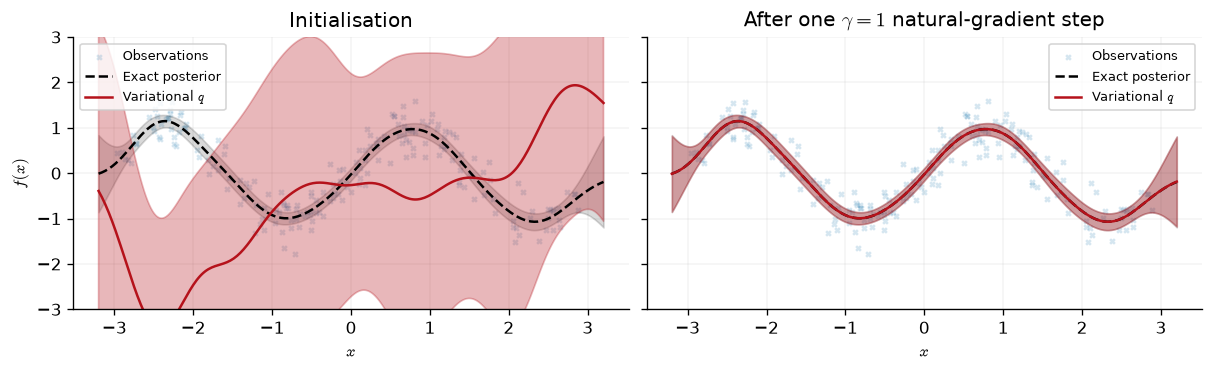
The right-hand panel is the point of the whole method: a single natural-gradient step has taken a deliberately absurd \(q\) onto the sparse variational optimum, which for \(M=20\) inducing points on this problem is not distinguishable by eye from the exact posterior. The printed maximum is taken over the whole test grid \([-3.2, 3.2]\) and is attained at its edge, past the last inducing input; restricted to the data range \([-3, 3]\) the two means agree roughly ten times more closely again. Both gaps are a fraction of a percent of the panel height, and both are a property of the sparse approximation, not of the optimiser.
Now the comparison. We freeze every hyperparameter with paramax.non_trainable — so
that both methods are solving the same problem, namely finding the best
\((\mathbf{m},\mathbf{L})\) for a fixed kernel — and run Adam on the variational
parameters from the same bad initialisation.
frozen_family = eqx.combine(
    variational_partition, paramax.non_trainable(hyper_partition)
)

adam_iterations = 2000
_, adam_history = gpx.fit(
    model=frozen_family,
    objective=negative_elbo,
    train_data=regression_data,
    optim=ox.adam(1e-2),
    num_iters=adam_iterations,
    key=jr.key(0),
    verbose=False,
)

adam_gap = jnp.asarray(adam_history) + reference_elbo
natgrad_gap = reference_elbo - stepped_elbo
iteration_index = jnp.arange(adam_gap.size)
for tolerance in [10.0, 1.0, 0.1]:
    first_hit = jnp.min(jnp.where(adam_gap < tolerance, iteration_index, adam_gap.size))
    reached = "never" if int(first_hit) == adam_gap.size else f"{int(first_hit)}"
    print(
        f"Adam iterations to come within {tolerance:5.1f} nats of the optimum: "
        f"{reached}"
    )
print(
    f"Adam ELBO gap after {adam_iterations} iterations : {float(adam_gap[-1]):.3e} nats"
)
print(f"Natural-gradient ELBO gap after 1 iteration: {natgrad_gap:.3e} nats")
Adam iterations to come within  10.0 nats of the optimum: 1514
Adam iterations to come within   1.0 nats of the optimum: never
Adam iterations to come within   0.1 nats of the optimum: never
Adam ELBO gap after 2000 iterations : 4.573e+00 nats
Natural-gradient ELBO gap after 1 iteration: 0.000e+00 nats
fig, axes = plt.subplots(ncols=2, figsize=(10, 3.0))

axes[0].plot(
    iteration_index + 1, -adam_history, color=cols[0], label="Adam on $(m, L)$"
)
axes[0].axhline(reference_elbo, color="black", linestyle="--", label="Exact optimum")
axes[0].scatter(
    [1], [stepped_elbo], color=cols[1], zorder=5, s=45, label="Natural gradient, 1 step"
)
axes[0].set(
    xscale="log",
    xlabel="Iteration",
    ylabel="ELBO",
    ylim=(reference_elbo - 250, reference_elbo + 25),
)
clean_legend(axes[0])

axes[1].plot(iteration_index + 1, adam_gap, color=cols[0], label="Adam on $(m, L)$")
axes[1].scatter(
    [1], [natgrad_gap], color=cols[1], zorder=5, s=45, label="Natural gradient, 1 step"
)
axes[1].set(
    xscale="log", yscale="log", xlabel="Iteration", ylabel="ELBO gap to optimum (nats)"
)
clean_legend(axes[1])
<Axes: xlabel='Iteration', ylabel='ELBO gap to optimum (nats)'>
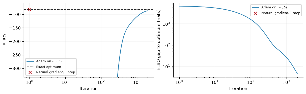
Read the right-hand panel rather than the left. On log-log axes Adam’s gap barely bends over the first few tens of iterations and then falls faster and faster, its slope steepest of all over the final few hundred — the opposite of the usual “fast start, long crawl” picture. That shape is the optimiser’s, not the problem’s: Adam normalises its step, so each coordinate moves by at most the learning rate however large the gradient is, and from an initialisation this bad it is the distance to be travelled that binds, not the gradient. The printed numbers say the same thing: more than a thousand iterations merely to come within ten nats of the optimum, and after two thousand it is still several nats short and still descending, while the single natural-gradient step closed the gap to around \(10^{-14}\) nats. Adam is converging; it is simply converging in coordinates that put the optimum a long way away. The natural gradient never travels that distance, because the Fisher metric rescales it.
Two caveats before this is oversold. The hyperparameters were frozen, so this is the problem natural gradients are best at: a pure variational optimisation. And the advantage rests on conjugacy, which is what makes \(\gamma=1\) a solve rather than a step. Neither holds in the next demo.
Non-conjugate models: ramping \(\gamma\)#
Outside conjugacy, \(\mathbb{E}_q[\log p(\mathbf{y}\mid\mathbf{u})]\) is no longer affine in \(\boldsymbol{\eta}\), so \(\gamma=1\) is no longer a solve — it is a large step along a direction that was only computed locally. Salimbeni et al. find experimentally that “the initial natural gradient step size is a small value that is parameterization and likelihood dependent, but then increases to \(\gamma = 1\)”, and in the stochastic setting they adopt a two-phase schedule: a log-linear ramp
Their reported settings are \(\gamma_{\text{init}}=10^{-4}\), \(\gamma_{\text{final}}=10^{-1}\) with \(K\) between 5 and 40 for UCI-scale problems at batch size 256, and \(\gamma_{\text{init}}=10^{-6}\), \(\gamma_{\text{final}}=2\times10^{-2}\), \(K=2000\) for MNIST at batch size 1024, always with \(\gamma^{\text{Adam}} = 10^{-2}\) on the hyperparameters. Their conclusion is that “the success of the method relies on \(\gamma\) increasing to a reasonably large value (\(\approx 0.1\)) sufficiently quickly (\(<1000\) iterations)”.
We use \(K = 100\) below. Their \(K\) is dataset-dependent — 5 for the smaller UCI sets, 40 for NAVAL, 2000 for MNIST — and \(100\) buys a little extra cone headroom (see the last section) at this \(M\) from the default \(\mathbf{m}=\mathbf{0}\), \(\mathbf{S}=\mathbf{I}\) start, while still satisfying their own \(<1000\)-iteration criterion.
Why does \(\gamma < 1\) help when mini-batching? The \(N/B\) rescaling inside the ELBO makes the stochastic gradient unbiased, and because \(\boldsymbol{\theta}_{\text{new}} = \boldsymbol{\theta} - \gamma\hat{\mathbf{g}}\) is affine in \(\hat{\mathbf{g}}\), \(\boldsymbol{\theta}_{\text{new}}\) is unbiased for the full-batch update at every \(\gamma\), including \(\gamma=1\). What degrades is variance. The step is always a combination \(\boldsymbol{\theta}_{\text{new}} = (1-\gamma)\,\boldsymbol{\theta} + \gamma\,\boldsymbol{\theta}^{\text{tgt}}\) — the failure-modes section below writes its second block out explicitly — but outside conjugacy \(\boldsymbol{\theta}^{\text{tgt}}\) is not a fixed optimum. It depends on the current \(q\) as well as on the current mini-batch: it is where one fixed-point iteration from here would land, and it moves as \(q\) moves. At \(\gamma=1\) the step discards \(\boldsymbol{\theta}_t\) entirely and jumps onto that noisy, moving target, so nothing averages the mini-batch noise out of it. Taking \(\gamma<1\) makes the update an exponential moving average in \(\boldsymbol{\theta}\) towards the target, and that is where the variance reduction comes from. A second, smaller effect compounds it: \(\boldsymbol{\theta}\mapsto(\mathbf{m},\mathbf{S})\) is nonlinear, so unbiasedness in \(\boldsymbol{\theta}\) does not survive the conversion back to moments.
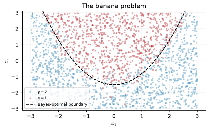
Time for a harder problem.
def make_banana(key, num_points):
    """Two-class banana problem with a curved Bayes-optimal boundary."""
    key_latent, key_label = jr.split(key)
    latent = jr.uniform(key_latent, (num_points, 2), minval=-3.0, maxval=3.0)
    decision = latent[:, 1] - (0.7 * latent[:, 0] ** 2 - 1.5)
    probability = jax.nn.sigmoid(3.0 * decision)
    labels = (jr.uniform(key_label, (num_points,)) < probability).astype(jnp.float64)
    return latent, labels[:, None]


banana_key = jr.key(42)
banana_inputs, banana_labels = make_banana(banana_key, 2000)
banana_data = gpx.Dataset(X=banana_inputs, y=banana_labels)

num_train = 1600
train_inputs, test_inputs_2d = banana_inputs[:num_train], banana_inputs[num_train:]
train_labels, test_labels = banana_labels[:num_train], banana_labels[num_train:]
banana_train = gpx.Dataset(X=train_inputs, y=train_labels)

print(f"train / test  : {banana_train.n} / {banana_data.n - banana_train.n}")
print(f"class balance : {float(banana_data.y.mean()):.3f}")
train / test  : 1600 / 400
class balance : 0.420
boundary_inputs = jnp.linspace(-3.0, 3.0, 200)
boundary_outputs = 0.7 * boundary_inputs**2 - 1.5

fig, ax = plt.subplots(figsize=(5.5, 3.4))
for label, colour, name in [(0.0, cols[0], "$y = 0$"), (1.0, cols[1], "$y = 1$")]:
    mask = banana_labels.ravel() == label
    ax.scatter(
        banana_inputs[mask, 0],
        banana_inputs[mask, 1],
        s=6,
        alpha=0.4,
        color=colour,
        label=name,
    )
ax.plot(
    boundary_inputs,
    boundary_outputs,
    color="black",
    linestyle="--",
    label="Bayes-optimal boundary",
)
ax.set(xlabel=r"$x_1$", ylabel=r"$x_2$", ylim=(-3.1, 3.1), title="The banana problem")
clean_legend(ax)
<Axes: title={'center': 'The banana problem'}, xlabel='$x_1$', ylabel='$x_2$'>
# Two identical models, built from the same arrays, so the comparison is fair.
num_banana_inducing = 50
inducing_grid = jnp.meshgrid(jnp.linspace(-2.8, 2.8, 10), jnp.linspace(-2.8, 2.8, 5))
banana_inducing = jnp.stack([axis.ravel() for axis in inducing_grid], axis=1)

banana_model = (
    gpx.gps.Prior(
        mean_function=gpx.mean_functions.Zero(), kernel=jk.RBF(active_dims=[0, 1])
    )
    * gpx.likelihoods.Bernoulli()
)


def make_banana_family():
    """A fresh SVGP over the banana data, at the default m = 0, S = I."""
    return gpx.variational_families.VariationalGaussian(
        model=banana_model, inducing_inputs=banana_inducing
    )


natgrad_family = make_banana_family()
adam_family = make_banana_family()

print(f"inducing inputs: {banana_inducing.shape}")
inducing inputs: (50, 2)
# The log-linear ramp, 1e-4 -> 1e-1 over K = 100 iterations, as an Optax schedule.
num_iterations = 1000
batch_size = 256
natgrad_schedule = ox.exponential_decay(
    init_value=1e-4, transition_steps=100, decay_rate=1000.0, end_value=1e-1
)
print(
    "gamma at iterations 0, 50, 100, 999: "
    + ", ".join(f"{float(natgrad_schedule(t)):.2e}" for t in [0, 50, 100, 999])
)


def timed_fit(run):
    """Run twice: the first call pays JIT compilation, the second is steady state."""
    model, history = run()
    history.block_until_ready()
    start = time.perf_counter()
    model, history = run()
    history.block_until_ready()
    return model, history, time.perf_counter() - start
gamma at iterations 0, 50, 100, 999: 1.00e-04, 3.16e-03, 1.00e-01, 1.00e-01
natgrad_model, natgrad_history, natgrad_seconds = timed_fit(
    lambda: gpx.fit_natgrads(
        model=natgrad_family,
        objective=negative_elbo,
        train_data=banana_train,
        optim=ox.adam(1e-2),
        natgrad_lr=natgrad_schedule,
        batch_size=batch_size,
        num_iters=num_iterations,
        key=jr.key(1),
        verbose=False,
    )
)
print(
    f"natural gradients + Adam : {natgrad_seconds:.2f} s "
    f"({1e3 * natgrad_seconds / num_iterations:.2f} ms / iteration)"
)
natural gradients + Adam : 4.48 s (4.48 ms / iteration)
adam_model, adam_banana_history, adam_seconds = timed_fit(
    lambda: gpx.fit(
        model=adam_family,
        objective=negative_elbo,
        train_data=banana_train,
        optim=ox.adam(1e-2),
        batch_size=batch_size,
        num_iters=num_iterations,
        key=jr.key(1),
        verbose=False,
    )
)
print(
    f"Adam only                : {adam_seconds:.2f} s "
    f"({1e3 * adam_seconds / num_iterations:.2f} ms / iteration)"
)
Adam only : 2.90 s (2.90 ms / iteration)
Both runs use ox.adam(1e-2) on the kernel hyperparameters and the inducing inputs,
so the only difference is how \((\mathbf{m},\mathbf{L})\) move. Timings are steady
state: each fit is called twice and only the second call is timed, so JIT
compilation is excluded from both. They were measured on CPU while executing this
notebook, and will differ on your machine.
smoothing_window = 25


def smooth(history):
    """Trailing mean over `smoothing_window` iterations."""
    return jnp.convolve(
        history, jnp.ones(smoothing_window) / smoothing_window, mode="valid"
    )


smoothed_iterations = jnp.arange(smoothing_window - 1, num_iterations)
smoothed_natgrad = smooth(natgrad_history)
smoothed_adam = smooth(adam_banana_history)

# Derive the axis limits from the curves, so nothing is silently clipped on a machine
# whose run lands somewhere else.
elbo_floor = 0.95 * float(jnp.minimum(smoothed_natgrad.min(), smoothed_adam.min()))
elbo_ceiling = 1.10 * float(jnp.maximum(smoothed_natgrad.max(), smoothed_adam.max()))

fig, axes = plt.subplots(ncols=2, figsize=(10, 3.0), sharey=True)
for ax, horizontal, xlabel in [
    (axes[0], smoothed_iterations, "Iteration"),
    (
        axes[1],
        jnp.linspace(0.0, natgrad_seconds, num_iterations)[smoothing_window - 1 :],
        "Wall-clock seconds",
    ),
]:
    ax.plot(
        horizontal, smoothed_natgrad, color=cols[1], label="Natural gradients + Adam"
    )
    ax.set(xlabel=xlabel, yscale="log", ylim=(elbo_floor, elbo_ceiling))
axes[0].plot(smoothed_iterations, smoothed_adam, color=cols[0], label="Adam only")
axes[1].plot(
    jnp.linspace(0.0, adam_seconds, num_iterations)[smoothing_window - 1 :],
    smoothed_adam,
    color=cols[0],
    label="Adam only",
)
axes[0].set_ylabel("Negative ELBO (mini-batch)")
clean_legend(axes[0])
clean_legend(axes[1])

target_value = float(smoothed_adam[-1])
# Sentinel above every attainable iteration index, so "never crossed" is distinguishable
# from "crossed on the last iteration".
never = num_iterations + 1
crossing = int(
    jnp.min(jnp.where(smoothed_natgrad < target_value, smoothed_iterations, never))
)
print(
    f"Adam only, negative ELBO after {num_iterations} iterations   : "
    f"{target_value:8.2f}"
)
if crossing == never:
    print("Natural gradients, same value reached at iteration : never")
else:
    print(f"Natural gradients, same value reached at iteration : {crossing}")
    print(
        f"  i.e. {crossing * natgrad_seconds / num_iterations:.2f} s "
        f"versus {adam_seconds:.2f} s"
    )
print(
    "Natural gradients, negative ELBO after "
    f"{num_iterations} iterations: {float(smoothed_natgrad[-1]):8.2f}"
)
Adam only, negative ELBO after 1000 iterations   :   335.31
Natural gradients, same value reached at iteration : 117
  i.e. 0.52 s versus 2.90 s
Natural gradients, negative ELBO after 1000 iterations:   323.98
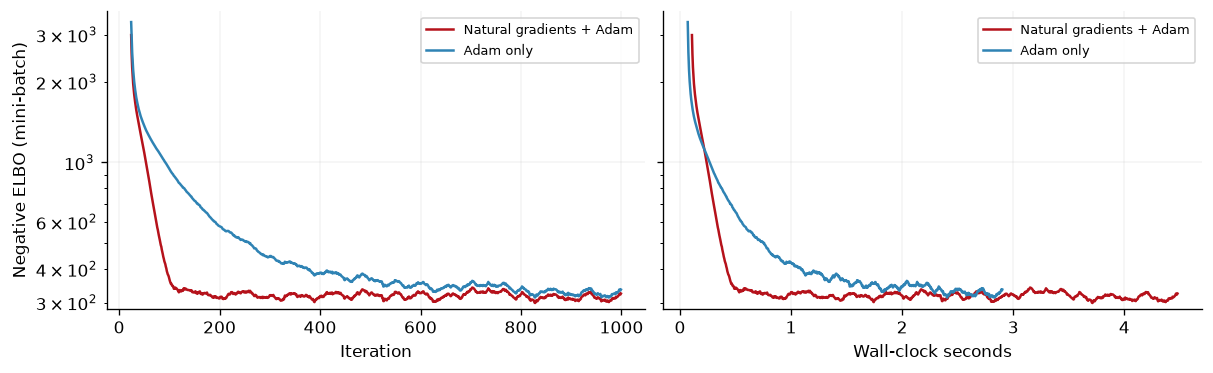
Both curves are mini-batch estimates and therefore noisy; they are shown as a 25-iteration trailing mean. Per iteration the natural-gradient run is far ahead. Per second it is still ahead, but by less, because each of its iterations does strictly more work: a natural-gradient step converts \((\mathbf{m},\mathbf{L})\) to \(\boldsymbol{\eta}\), differentiates the loss through the inverse map, converts back through \(\boldsymbol{\theta}\), and then takes the Adam step on the hyperparameters. On the CPU that rendered this page that came to roughly half again the cost per iteration — see the timings printed above, which are what your machine actually measured. Salimbeni et al. report a comparable ratio of about \(1.5\times\), and their headline experiments are on datasets far larger than this one; treat the numbers here as a demonstration of the mechanism, not as a benchmark.
grid_side = 64
grid_axis = jnp.linspace(-3.1, 3.1, grid_side)
grid_x, grid_y = jnp.meshgrid(grid_axis, grid_axis)
grid_points = jnp.stack([grid_x.ravel(), grid_y.ravel()], axis=1)


def predictive_probability(model, inputs, num_chunks=8):
    """Bernoulli success probability, evaluated in chunks to bound memory."""
    unwrapped = paramax.unwrap(model)
    likelihood = unwrapped.model.likelihood
    return jnp.concatenate(
        [likelihood(unwrapped(chunk)).mean for chunk in jnp.split(inputs, num_chunks)]
    )


fig, axes = plt.subplots(ncols=2, figsize=(10, 3.6), sharey=True)
for ax, model, name, seconds in [
    (axes[0], natgrad_model, "Natural gradients + Adam", natgrad_seconds),
    (axes[1], adam_model, "Adam only", adam_seconds),
]:
    probability = predictive_probability(model, grid_points).reshape(
        grid_side, grid_side
    )
    contours = ax.contourf(
        grid_x,
        grid_y,
        probability,
        levels=jnp.linspace(0.0, 1.0, 11),
        cmap="RdBu_r",
        alpha=0.7,
    )
    ax.contour(
        grid_x, grid_y, probability, levels=[0.5], colors="black", linewidths=1.5
    )
    ax.plot(
        boundary_inputs, boundary_outputs, color="black", linestyle="--", linewidth=1
    )
    # Held-out points, encoded by class in the notebook's categorical colours rather
    # than in the contour colourmap, so they stay legible on top of the fill.
    for label, colour, marker in [(0.0, cols[0], "o"), (1.0, cols[1], "^")]:
        mask = test_labels.ravel() == label
        ax.scatter(
            test_inputs_2d[mask, 0],
            test_inputs_2d[mask, 1],
            marker=marker,
            s=12,
            alpha=0.9,
            color=colour,
            edgecolors="white",
            linewidths=0.3,
        )
    inducing = paramax.unwrap(model).inducing_inputs
    ax.scatter(inducing[:, 0], inducing[:, 1], marker="+", s=25, color="black")

    probability_test = predictive_probability(model, test_inputs_2d, num_chunks=1)
    accuracy = jnp.mean((probability_test > 0.5) == (test_labels.ravel() > 0.5))
    log_density = jnp.mean(
        test_labels.ravel() * jnp.log(probability_test)
        + (1.0 - test_labels.ravel()) * jnp.log1p(-probability_test)
    )
    ax.set(
        xlabel=r"$x_1$",
        xlim=(-3.1, 3.1),
        ylim=(-3.1, 3.1),
        title=f"{name}\naccuracy {accuracy:.3f}, NLPD {-log_density:.3f}",
    )
    print(
        f"{name:26s} test accuracy {accuracy:.4f}, test NLPD {-log_density:.4f}, "
        f"{seconds:.2f} s"
    )
axes[0].set_ylabel(r"$x_2$")
colourbar = fig.colorbar(contours, ax=axes, label=r"$q(y=1 \mid x)$")
Natural gradients + Adam   test accuracy 0.9350, test NLPD 0.1663, 4.48 s
Adam only                  test accuracy 0.9325, test NLPD 0.1694, 2.90 s
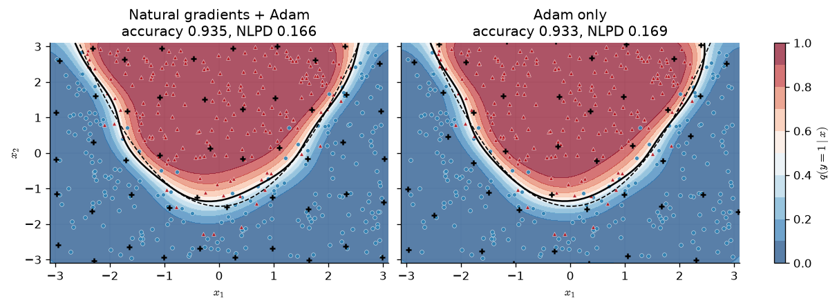
The solid black line is each model’s \(0.5\) contour and the dashed line is the Bayes-optimal boundary \(x_2 = 0.7x_1^2 - 1.5\); crosses mark the inducing inputs after training.
The two panels are very nearly the same picture, and the two sets of printed test
metrics are very nearly the same numbers. That is the honest reading of this
experiment, and it is worth stating plainly: on a densely-sampled, easily-separated
problem the natural gradient buys optimiser speed, not final predictive quality. It
reached Adam’s thousand-iteration bound at the crossing iteration printed under the
ELBO comparison above, and both models then classify the held-out points about
equally well. Note also
that both runs train the kernel and the inducing inputs with Adam and finish at
different hyperparameters, so whatever small difference remains between these
contours cannot be attributed to \(\mathbf{S}\) alone. make_banana draws inputs
uniformly on \([-3,3]^2\) and the plotted grid is \([-3.1,3.1]^2\), so there is no
region here that is far from the data; a demonstration that natural gradients give
better-calibrated extrapolative uncertainty would need a problem built for it.
When natural gradients fail#
The step is \(\boldsymbol{\theta}\leftarrow\boldsymbol{\theta} - \gamma\,\partial\ell/\partial\boldsymbol{\eta}\), and \(\boldsymbol{\Theta}_2\) must stay negative definite, because \(\boldsymbol{\Theta}_2 = -\tfrac12\mathbf{S}^{-1}\) and \(\mathbf{S}\) is a covariance. Nothing in the update enforces that. Splitting the ELBO as \(\mathcal{L} = \mathcal{L}_{\text{data}} - \operatorname{KL}[q\,\|\,p]\) and using \(\partial\operatorname{KL}/\partial\mathbf{S} = \tfrac12\mathbf{K}_{zz}^{-1} - \tfrac12\mathbf{S}^{-1}\) gives an exact description of what happens:
(for the whitened family, replace \(\mathbf{K}_{zz}^{-1}\) by \(\mathbf{I}_M\)). So the step is a convex combination in \(\boldsymbol{\theta}\)-space whenever \(\gamma\in[0,1]\) — the mirror-descent reading, made concrete.
Cone-safety theorem. If the likelihood is log-concave in \(f\), then by Price’s theorem (\(\partial_{\mathbf{S}}\mathbb{E}_{\mathcal{N}(\mathbf{m},\mathbf{S})}[g] = \tfrac12\mathbb{E}[\nabla^2 g]\)),
where \(\mathbf{a}_n^\top\) is row \(n\) of \(\mathbf{A} = \mathbf{K}_{xz}\mathbf{K}_{zz}^{-1}\). Hence \(\boldsymbol{\Theta}_2^{\text{tgt}} \prec 0\), and for \(\gamma\in[0,1]\) \(\boldsymbol{\Theta}_2^{\text{new}}\) is a convex combination of two negative-definite matrices, so it is negative definite. Mini-batching does not break this, because \(N/B > 0\) preserves the sign. \(\square\)
Two things escape the theorem: \(\gamma > 1\), which extrapolates past
\(\boldsymbol{\Theta}_2^{\text{tgt}}\); and likelihoods that are not log-concave
(Student-\(t\), for instance), for which
\(\partial\mathcal{L}_{\text{data}}/\partial\mathbf{S}\) can have positive eigenvalues
and the target itself sits outside the cone. Log-concavity here is a property of the
likelihood as computed, not as written: GPJax’s inv_probit clips its output into
\([10^{-3},\,1-10^{-3}]\), which flattens the tail of \(\log p\) enough to give it a
positive second derivative for \(f \lesssim -2.44\), so even the Bernoulli model used
below leaves the guaranteed regime once a point is confidently mislabelled. That is
the behaviour the backoff below is really guarding. Below we sweep \(\gamma\) from an
over-confident starting point — \(\mathbf{S}_0 = 10^{-2}\mathbf{I}\), sharper than the
target — which is precisely the regime where extrapolation bites.
overconfident_family = gpx.variational_families.VariationalGaussian(
    model=banana_model,
    inducing_inputs=banana_inducing,
    variational_mean=jnp.zeros((num_banana_inducing, 1)),
    variational_root_covariance=0.1 * jnp.eye(num_banana_inducing),
)
overconfident_mean = overconfident_family.variational_mean.unwrap()
overconfident_root = overconfident_family.variational_root_covariance.unwrap()


def banana_loss_of_expectation(expectation):
    variational_mean, variational_root = moments_from_expectation(*expectation)
    trial = eqx.tree_at(
        lambda family: (family.variational_mean, family.variational_root_covariance),
        overconfident_family,
        (Real(variational_mean), LowerTriangular(variational_root)),
    )
    return negative_elbo(paramax.unwrap(trial), banana_train)


cone_gradient = jax.grad(banana_loss_of_expectation)(
    expectation_from_moments(overconfident_mean, overconfident_root)
)
# The matrix statistic is symmetric, so symmetrise the entrywise autodiff gradient.
matrix_gradient = 0.5 * (cone_gradient[1] + cone_gradient[1].T)
_, natural_matrix = natural_from_moments(overconfident_mean, overconfident_root)

print("gamma      max eig(Theta2_new)   status")
for gamma in [0.1, 0.5, 1.0, 2.0, 5.0, 10.0]:
    largest = jnp.max(jnp.linalg.eigvalsh(natural_matrix - gamma * matrix_gradient))
    status = "negative definite" if largest < 0 else "*** LEFT THE CONE ***"
    print(f"{gamma:6.2f}   {largest:+18.5f}   {status}")
gamma      max eig(Theta2_new)   status
  0.10            -45.46684   negative definite
  0.50            -27.33418   negative definite
  1.00             -4.66836   negative definite
  2.00            +40.66328   *** LEFT THE CONE ***
  5.00           +176.65821   *** LEFT THE CONE ***
 10.00           +403.31642   *** LEFT THE CONE ***
Read that table as a statement about this initialisation, not about \(\gamma=2\). Here \(\mathbf{S}_0 = 10^{-2}\mathbf{I}\) makes \(\boldsymbol{\Theta}_2 = -50\,\mathbf{I}\), an order of magnitude sharper than the target, so the convex combination has very little room to extrapolate into. Because \(\boldsymbol{\Theta}_2\) is a multiple of the identity, \(\lambda_{\max}(\boldsymbol{\Theta}_2^{\text{new}})\) is exactly linear in \(\gamma\), and interpolating the printed \(\gamma=1\) and \(\gamma=2\) rows puts the crossing at \(\gamma\approx1.1\). Where it lands is entirely a function of how far \(\boldsymbol{\Theta}_2\) starts from \(\boldsymbol{\Theta}_2^{\text{tgt}}\): in the limit where the two coincide, every \(\gamma\) is safe. What the theorem actually guarantees is \(\gamma\in[0,1]\), for any log-concave likelihood and any starting point, and it says nothing whatsoever beyond that — which is the line worth remembering.
When it does go wrong, jnp.linalg.cholesky returns NaN rather than raising,
which means validity is a value and the fix stays jit-compatible.
natural_gradient_step exploits that with a backoff: it evaluates the trial steps
\(\{\gamma\beta^k\}_{k=0}^{K}\) under vmap and selects the first one whose Cholesky
is finite. backoff (\(\beta\), default \(0.5\)) and max_backoff (\(K\), default \(5\))
are exposed by fit_natgrads.
print("gamma = 100 from the over-confident initialisation")
overconfident_variational, overconfident_hyper = partition_variational(
    overconfident_family
)
for max_backoff in [0, 3, 5, 7, 10]:
    stepped, _ = natural_gradient_step(
        overconfident_variational,
        overconfident_hyper,
        banana_train,
        negative_elbo,
        100.0,
        max_backoff=max_backoff,
    )
    smallest_trial = 100.0 * 0.5**max_backoff
    root = eqx.combine(
        stepped, overconfident_hyper
    ).variational_root_covariance.unwrap()
    outcome = "finite" if bool(jnp.all(jnp.isfinite(root))) else "NaN"
    print(
        f"  max_backoff = {max_backoff:2d}  smallest trial gamma = "
        f"{smallest_trial:7.3f}   result: {outcome}"
    )
gamma = 100 from the over-confident initialisation
  max_backoff =  0  smallest trial gamma = 100.000   result: NaN
  max_backoff =  3  smallest trial gamma =  12.500   result: NaN
  max_backoff =  5  smallest trial gamma =   3.125   result: NaN
  max_backoff =  7  smallest trial gamma =   0.781   result: finite
  max_backoff = 10  smallest trial gamma =   0.098   result: finite
The backoff is a safety net with a finite budget, not a licence to pick \(\gamma\)
carelessly: from this starting point it needs to shrink \(\gamma=100\) by a factor of
\(2^7\) before the Cholesky succeeds, so the default max_backoff=5 still returns
NaN. That is the intended behaviour — a silent 32-fold reduction of a step size the
user chose badly would be worse than a visible failure.
Practical guidance#
Conjugate and full batch: use \(\gamma = 1\). One iteration is the exact solution, and further iterations are fixed points.
Non-conjugate or mini-batched: ramp \(\gamma\). Salimbeni et al. recommend starting around \(10^{-4}\) and reaching \(\approx 10^{-1}\) “sufficiently quickly (\(<1000\) iterations)”;
natgrad_lraccepts any Optax schedule, and defaults to \(10^{-1}\).Never exceed \(\gamma = 1\). The convex-combination guarantee stops there, and the backoff exists to catch mistakes, not to enable them.
If a mini-batched run produces
NaN, raise the batch size before lowering \(\gamma\). Small batches make \(\boldsymbol{\Theta}_2^{\text{tgt}}\) badly conditioned, which no step size fully repairs.Prefer the whitened family. The natural-gradient direction is parameterisation-invariant, so whitening does not change the sequence of distributions in exact arithmetic; it changes the conditioning of every map, and keeps \(\mathbf{m}_w\), \(\mathbf{S}_w\) at \(\mathcal{O}(1)\).
Leave
map_jitterat \(0\). It biases \(\mathbf{S}\) by \(\approx\varepsilon\lVert\mathbf{S}\rVert^2\) independently of conditioning. Raise it to \(10^{-12}\)–\(10^{-10}\) only when fighting an ill-conditioned \(\mathbf{S}\).Non-log-concave likelihoods have no guarantee at all. For a Student-\(t\) likelihood with gross outliers the target \(\boldsymbol{\Theta}_2^{\text{tgt}}\) can itself be outside the cone, so no positive \(\gamma\) is provably safe.
The companion dual sparse GP notebook takes the same geometry in a different direction, storing the site parameters of the variational distribution rather than its moments.
System configuration#
%reload_ext watermark
%watermark -n -u -v -iv -w -a 'Thomas Pinder'
Author: Thomas Pinder

Last updated: Fri, 07 Aug 2026

Python implementation: CPython
Python version       : 3.11.15
IPython version      : 9.15.0

equinox   : 0.13.8
gpjax     : 0.18.0
jax       : 0.10.2
jaxtyping : 0.3.11
matplotlib: 3.11.1
optax     : 0.2.8
paramax   : 0.0.5

Watermark: 2.6.0