Multi-Output Gaussian Processes#
Download this notebook: multioutput.ipynb
Standard Gaussian process models, such as the one built in the regression notebook, map a \(D\)-dimensional input to a single scalar output. In many settings, however, we wish to model several correlated output quantities simultaneously. A multi-output Gaussian process captures these correlations so that observations of one output can inform predictions of another.
This notebook introduces the Intrinsic Coregionalization Model (ICM) implemented in GPJax. We construct a synthetic dataset with two correlated outputs, fit an ICM model by optimising the marginal log-likelihood, and inspect the learned coregionalization matrix to see what the model has discovered about the output structure.
from utils import use_mpl_style
from jax import config
import jax.numpy as jnp
import jax.random as jr
from jaxtyping import install_import_hook
import matplotlib as mpl
import matplotlib.pyplot as plt

config.update("jax_enable_x64", True)

with install_import_hook("gpjax", "beartype.beartype"):
    import gpjax as gpx

key = jr.key(42)
use_mpl_style()
cols = mpl.rcParams["axes.prop_cycle"].by_key()["color"]
The Intrinsic Coregionalization Model#
The ICM assumes that all outputs share a single latent Gaussian process, weighted differently for each output through a positive semi-definite coregionalization matrix \(\mathbf{B} \in \mathbb{R}^{P \times P}\). Given an input-space kernel \(k(\mathbf{x}, \mathbf{x}')\), the multi-output covariance between output \(p\) at input \(\mathbf{x}\) and output \(q\) at input \(\mathbf{x}'\) is
Stacking all \(N\) observations across \(P\) outputs into a single vector of length \(NP\), the joint covariance matrix takes the Kronecker form
where \(\mathbf{K}_{\mathbf{x}\mathbf{x}}\) is the \(N \times N\) Gram matrix of the base kernel.
The coregionalization matrix is parameterised as
where \(\mathbf{W} \in \mathbb{R}^{P \times R}\) is a low-rank factor of rank \(R\) and \(\boldsymbol{\kappa} \in \mathbb{R}^P_{>0}\) is a positive diagonal. The rank parameter controls how many latent sources of correlation the model can express. When \(R = 1\) and \(P = 2\), the model captures a single shared direction of variation between the two outputs.
Synthetic dataset#
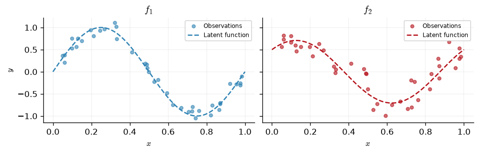
We generate two correlated functions on the interval \([0, 1]\). The first output is \(f_1(x) = \sin(2\pi x)\) and the second is a mixture \(f_2(x) = 0.5\sin(2\pi x) + 0.5\cos(2\pi x)\), so the two outputs share a sinusoidal component. Both are corrupted by Gaussian noise with different standard deviations (\(\sigma_1 = 0.1\), \(\sigma_2 = 0.2\)) to illustrate the per-output noise capability of the multi-output likelihood.
N = 40
P = 2
noise_stds = jnp.array([0.1, 0.2])

key, subkey1, subkey2 = jr.split(key, 3)
x = jnp.sort(jr.uniform(subkey1, shape=(N,), minval=0.0, maxval=1.0)).reshape(-1, 1)

f1 = lambda x: jnp.sin(2 * jnp.pi * x)
f2 = lambda x: 0.5 * f1(x) + 0.5 * jnp.cos(2 * jnp.pi * x)

y1 = f1(x) + jr.normal(subkey1, shape=x.shape) * noise_stds[0]
y2 = f2(x) + jr.normal(subkey2, shape=x.shape) * noise_stds[1]
y = jnp.hstack([y1, y2])  # [N, 2]

D = gpx.Dataset(X=x, y=y)
We plot the two outputs alongside the latent functions that generated them.
xtest = jnp.linspace(0.0, 1.0, 200).reshape(-1, 1)
output_labels = [r"$f_1$", r"$f_2$"]
latent_fns = [f1, f2]

fig, axes = plt.subplots(1, 2, figsize=(8, 2.5), sharey=True)

for i, ax in enumerate(axes):
    ax.plot(x, y[:, i], "o", color=cols[i], alpha=0.6, label="Observations", ms=4)
    ax.plot(
        xtest, latent_fns[i](xtest), color=cols[i], ls="--", label="Latent function"
    )
    ax.set_title(output_labels[i])
    ax.set_xlabel(r"$x$")
    ax.legend(loc="best", fontsize=7)

axes[0].set_ylabel(r"$y$")
Text(0, 0.5, '$y$')
Model definition#
We construct the ICM model in three steps. First, we build a
CoregionalizationMatrix with
\(P = 2\) outputs and rank \(R = 1\). Second, we wrap an RBF base kernel together
with the coregionalization matrix inside an
ICMKernel. Third, we pair a zero-mean GP prior
with a MultiOutputGaussian
likelihood, which allows a separate noise variance for each output.
key, subkey = jr.split(key)

coreg = gpx.parameters.CoregionalizationMatrix(num_outputs=P, rank=1, key=subkey)
kernel = gpx.kernels.ICMKernel(
    base_kernel=gpx.kernels.RBF(),
    coregionalization_matrix=coreg,
)

meanf = gpx.mean_functions.Zero()
prior = gpx.gps.Prior(mean_function=meanf, kernel=kernel)
likelihood = gpx.likelihoods.MultiOutputGaussian(
    num_outputs=P, obs_stddev=1.0
)
posterior = prior * likelihood
Before optimisation we verify that the marginal log-likelihood is finite.
print(f"Initial negative MLL: {-gpx.objectives.conjugate_mll(posterior, D):.3f}")
Initial negative MLL: 87.658
Optimisation#
We optimise the kernel hyperparameters, the coregionalization matrix entries, and
the per-output noise standard deviations by maximising the conjugate marginal
log-likelihood using L-BFGS via fit_scipy.
opt_posterior, history = gpx.fit_scipy(
    model=posterior,
    objective=lambda p, d: -gpx.objectives.conjugate_mll(p, d),
    train_data=D,
)

print(f"Optimised negative MLL: {-gpx.objectives.conjugate_mll(opt_posterior, D):.3f}")
Optimization terminated successfully.
         Current function value: -14.234924
         Iterations: 21
         Function evaluations: 24
         Gradient evaluations: 24
Optimised negative MLL: -14.235
Prediction#
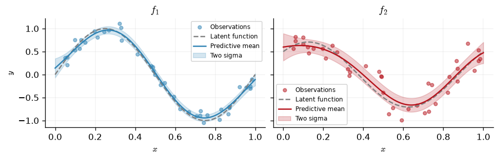
The multi-output posterior returns predictions as a single Gaussian distribution over a flattened vector of length \(MP\), where \(M\) is the number of test points and \(P\) is the number of outputs. The ordering is output-major: all \(M\) values for output 1 appear first, followed by all \(M\) values for output 2, and so on. We reshape the mean and extract per-output marginal variances from the diagonal of the joint covariance.
M = xtest.shape[0]
pred = opt_posterior.predict(xtest, train_data=D)

pred_mean = pred.mean.reshape(P, M).T  # [M, P]
pred_var = jnp.diag(pred.covariance()).reshape(P, M).T  # [M, P]
pred_std = jnp.sqrt(pred_var)
We now plot the predictive distribution for each output. The shaded region shows the predictive uncertainty of the model.
fig, axes = plt.subplots(1, 2, figsize=(8, 2.5), sharey=True)

for i, ax in enumerate(axes):
    ax.plot(x, y[:, i], "o", color=cols[i], alpha=0.5, label="Observations", ms=4)
    ax.plot(xtest, latent_fns[i](xtest), ls="--", color="grey", label="Latent function")
    ax.plot(xtest, pred_mean[:, i], color=cols[i], label="Predictive mean")
    ax.fill_between(
        xtest.squeeze(),
        pred_mean[:, i] - 2 * pred_std[:, i],
        pred_mean[:, i] + 2 * pred_std[:, i],
        color=cols[i],
        alpha=0.2,
        label="Two sigma",
    )
    ax.set_title(output_labels[i])
    ax.set_xlabel(r"$x$")
    ax.legend(loc="best", fontsize=7)

axes[0].set_ylabel(r"$y$")
Text(0, 0.5, '$y$')
Learned coregionalization matrix#
The coregionalization matrix \(\mathbf{B}\) encodes the learned correlations between outputs. Its off-diagonal entries indicate how strongly the outputs covary: a large positive entry between outputs \(p\) and \(q\) means they tend to increase together, while a value near zero suggests they are largely independent given the shared input kernel.
We visualise \(\mathbf{B}\) as a heatmap and print its entries.
B_learned = opt_posterior.prior.kernel.coregionalization_matrix.B

fig, ax = plt.subplots(figsize=(3.5, 3))
im = ax.imshow(
    B_learned,
    cmap="RdBu_r",
    vmin=-jnp.max(jnp.abs(B_learned)),
    vmax=jnp.max(jnp.abs(B_learned)),
)

for row in range(P):
    for col in range(P):
        ax.text(
            col,
            row,
            f"{B_learned[row, col]:.3f}",
            ha="center",
            va="center",
            fontsize=10,
        )

ax.set_xticks(range(P))
ax.set_yticks(range(P))
ax.set_xticklabels(output_labels)
ax.set_yticklabels(output_labels)
ax.set_title(r"Learned $\mathbf{B}$")
fig.colorbar(im, ax=ax, shrink=0.8)
<matplotlib.colorbar.Colorbar at 0x7fe8e81cec90>
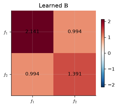
Because \(f_2\) is defined as a mixture that includes a scaled copy of \(f_1\), we expect the model to recover a positive correlation between the two outputs. The diagonal entries reflect each output’s marginal variance contribution from the shared latent process.
From ICM to LCM#
The Intrinsic Coregionalization Model is powerful but limited: it assumes that all inter-output correlations are explained by a single shared latent Gaussian process. When the outputs are driven by multiple independent sources of variation — for example, a slow trend and a fast oscillation — a single latent kernel cannot capture both length-scales simultaneously. The ICM must compromise, and the resulting fit degrades.
The Linear Model of Coregionalization (LCM) removes this limitation by combining \(Q\) independent latent GPs, each equipped with its own input-space kernel and its own output-space coregionalization matrix. The additional components give the model the flexibility to assign distinct spectral characteristics to different sources of inter-output coupling.
The Linear Model of Coregionalization#
Given \(Q\) latent kernels \(\{k_q\}_{q=1}^{Q}\) and \(Q\) coregionalization matrices \(\{\mathbf{B}^{(q)}\}_{q=1}^{Q}\), each of size \(P \times P\), the LCM defines the multi-output covariance between output \(p\) at input \(\mathbf{x}\) and output \(r\) at input \(\mathbf{x}'\) as
Stacking all \(N\) observations across \(P\) outputs into a single vector of length \(NP\), the joint covariance matrix is the sum of Kronecker products
where \(\mathbf{K}^{(q)}_{\mathbf{x}\mathbf{x}}\) is the \(N \times N\) Gram matrix of the \(q\)-th latent kernel.
Relationship to ICM#
Setting \(Q = 1\) recovers the ICM exactly: there is one kernel, one
coregionalization matrix, and the covariance has pure Kronecker structure. GPJax
exploits this: when an LCMKernel has a single
component, the compute engine returns a
Kronecker operator, preserving the efficient
\(\mathcal{O}(N^3 + P^3)\) decomposition. For \(Q > 1\) the sum of Kronecker
products no longer admits a
closed-form Kronecker inverse, so GPJax materialises the full \(NP \times NP\) dense
matrix and solves via a standard Cholesky factorisation in
\(\mathcal{O}((NP)^3)\). When \(P\) is large enough for that cost to bite, the
OILMM notebook shows a mixing-matrix parameterisation whose cost is
independent of \(P\) altogether.
Per-component coregionalization#
Each coregionalization matrix is parameterised as before:
where \(\mathbf{W}^{(q)} \in \mathbb{R}^{P \times R_q}\) is a low-rank factor and \(\boldsymbol{\kappa}^{(q)} \in \mathbb{R}^P_{>0}\) a positive diagonal. The rank \(R_q\) of each component can be chosen independently. A component with rank 1 captures one direction of inter-output correlation at the length-scale determined by \(k_q\); increasing the rank allows richer coupling patterns at that scale.
A three-output synthetic dataset#
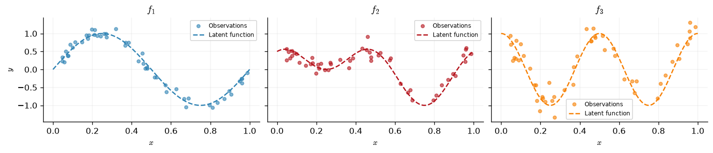
To demonstrate the advantage of multiple latent components, we construct a dataset with three outputs driven by two distinct latent functions:
\(g_1(x) = \sin(2\pi x)\) — a smooth, low-frequency oscillation,
\(g_2(x) = \cos(4\pi x)\) — a faster oscillation at double the frequency.
The three observed outputs are mixtures of these latent functions:
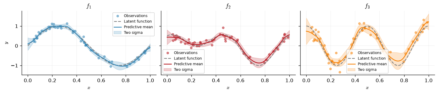
Outputs 1 and 3 are each dominated by a single latent source, while output 2 is a balanced mixture of both. A single-component ICM kernel would struggle here because it cannot separate the two frequency scales. An LCM with \(Q = 2\) components — each learning a different length-scale — should recover the latent structure.
N_lcm = 50
P_lcm = 3
noise_stds_lcm = jnp.array([0.1, 0.15, 0.2])

key, subkey1, subkey2, subkey3 = jr.split(key, 4)
x_lcm = jnp.sort(jr.uniform(subkey1, shape=(N_lcm,), minval=0.0, maxval=1.0)).reshape(
    -1, 1
)

g1 = lambda x: jnp.sin(2 * jnp.pi * x)
g2 = lambda x: jnp.cos(4 * jnp.pi * x)

f1_lcm = lambda x: g1(x)
f2_lcm = lambda x: 0.5 * g1(x) + 0.5 * g2(x)
f3_lcm = lambda x: g2(x)

y1_lcm = f1_lcm(x_lcm) + jr.normal(subkey1, shape=x_lcm.shape) * noise_stds_lcm[0]
y2_lcm = f2_lcm(x_lcm) + jr.normal(subkey2, shape=x_lcm.shape) * noise_stds_lcm[1]
y3_lcm = f3_lcm(x_lcm) + jr.normal(subkey3, shape=x_lcm.shape) * noise_stds_lcm[2]
y_lcm = jnp.hstack([y1_lcm, y2_lcm, y3_lcm])  # [N, 3]

D_lcm = gpx.Dataset(X=x_lcm, y=y_lcm)
We plot the three outputs alongside their latent functions.
xtest_lcm = jnp.linspace(0.0, 1.0, 200).reshape(-1, 1)
output_labels_lcm = [r"$f_1$", r"$f_2$", r"$f_3$"]
latent_fns_lcm = [f1_lcm, f2_lcm, f3_lcm]

fig, axes = plt.subplots(1, 3, figsize=(12, 2.5), sharey=True)

for i, ax in enumerate(axes):
    ax.plot(
        x_lcm, y_lcm[:, i], "o", color=cols[i], alpha=0.6, label="Observations", ms=4
    )
    ax.plot(
        xtest_lcm,
        latent_fns_lcm[i](xtest_lcm),
        color=cols[i],
        ls="--",
        label="Latent function",
    )
    ax.set_title(output_labels_lcm[i])
    ax.set_xlabel(r"$x$")
    ax.legend(loc="best", fontsize=7)

axes[0].set_ylabel(r"$y$")
Text(0, 0.5, '$y$')
LCM model definition#
We build an LCM with \(Q = 2\) components. The first component uses an RBF kernel,
which is well-suited to capture the smooth, low-frequency latent function \(g_1\).
The second component uses a Matérn-3/2 kernel, whose shorter default length-scale
can adapt to the faster oscillation in \(g_2\). Our
introduction to kernels compares the two families and the
sample paths each admits. Each component has its own
CoregionalizationMatrix with \(P = 3\) outputs and rank \(R = 1\), so each component
captures one direction of inter-output correlation at its characteristic
length-scale.
key, subkey1, subkey2 = jr.split(key, 3)

coreg1 = gpx.parameters.CoregionalizationMatrix(num_outputs=P_lcm, rank=1, key=subkey1)
coreg2 = gpx.parameters.CoregionalizationMatrix(num_outputs=P_lcm, rank=1, key=subkey2)

lcm_kernel = gpx.kernels.LCMKernel(
    kernels=[gpx.kernels.RBF(), gpx.kernels.Matern32()],
    coregionalization_matrices=[coreg1, coreg2],
)

meanf_lcm = gpx.mean_functions.Zero()
prior_lcm = gpx.gps.Prior(mean_function=meanf_lcm, kernel=lcm_kernel)
likelihood_lcm = gpx.likelihoods.MultiOutputGaussian(
    num_outputs=P_lcm, obs_stddev=1.0
)
posterior_lcm = prior_lcm * likelihood_lcm
Before optimisation we verify that the marginal log-likelihood is finite.
print(
    f"Initial negative MLL: {-gpx.objectives.conjugate_mll(posterior_lcm, D_lcm):.3f}"
)
Initial negative MLL: 167.936
Optimisation#
As with the ICM example, we maximise the conjugate marginal log-likelihood using
fit_scipy. The optimiser now has more parameters to tune: two sets of kernel
hyperparameters and two coregionalization matrices.
opt_posterior_lcm, history_lcm = gpx.fit_scipy(
    model=posterior_lcm,
    objective=lambda p, d: -gpx.objectives.conjugate_mll(p, d),
    train_data=D_lcm,
)

print(
    "Optimised negative MLL: "
    f"{-gpx.objectives.conjugate_mll(opt_posterior_lcm, D_lcm):.3f}"
)
Optimization terminated successfully.
         Current function value: -20.719374
         Iterations: 149
         Function evaluations: 177
         Gradient evaluations: 177
Optimised negative MLL: -20.719
Prediction#
The multi-output posterior returns predictions as a single Gaussian distribution over a flattened vector of length \(MP\), where \(M\) is the number of test points. The ordering is output-major: all \(M\) values for output 1 appear first, then output 2, then output 3. We reshape accordingly.
M_lcm = xtest_lcm.shape[0]
pred_lcm = opt_posterior_lcm.predict(xtest_lcm, train_data=D_lcm)

pred_mean_lcm = pred_lcm.mean.reshape(P_lcm, M_lcm).T
pred_var_lcm = jnp.diag(pred_lcm.covariance()).reshape(P_lcm, M_lcm).T
pred_std_lcm = jnp.sqrt(pred_var_lcm)
We now plot the predictive distribution for each of the three outputs. The shaded region shows the predictive uncertainty.
fig, axes = plt.subplots(1, 3, figsize=(12, 2.5), sharey=True)

for i, ax in enumerate(axes):
    ax.plot(
        x_lcm, y_lcm[:, i], "o", color=cols[i], alpha=0.5, label="Observations", ms=4
    )
    ax.plot(
        xtest_lcm,
        latent_fns_lcm[i](xtest_lcm),
        ls="--",
        color="grey",
        label="Latent function",
    )
    ax.plot(xtest_lcm, pred_mean_lcm[:, i], color=cols[i], label="Predictive mean")
    ax.fill_between(
        xtest_lcm.squeeze(),
        pred_mean_lcm[:, i] - 2 * pred_std_lcm[:, i],
        pred_mean_lcm[:, i] + 2 * pred_std_lcm[:, i],
        color=cols[i],
        alpha=0.2,
        label="Two sigma",
    )
    ax.set_title(output_labels_lcm[i])
    ax.set_xlabel(r"$x$")
    ax.legend(loc="best", fontsize=7)

axes[0].set_ylabel(r"$y$")
Text(0, 0.5, '$y$')
Learned coregionalization structure#
Unlike the ICM, which produces a single \(\mathbf{B}\) matrix, the LCM yields one coregionalization matrix per component. Each \(\mathbf{B}^{(q)}\) tells us how the \(q\)-th latent process couples the outputs. By inspecting these matrices we can recover which outputs share each latent source.
We expect the component paired with the RBF kernel (smooth, low-frequency) to show strong coupling between outputs 1 and 2, since both contain \(g_1\). The Matérn-3/2 component (higher frequency) should couple outputs 2 and 3, which share \(g_2\).
kernel_names = ["RBF (component 1)", "Matérn-3/2 (component 2)"]
fig, axes_B = plt.subplots(1, 2, figsize=(8, 3))

for idx, (cm, _k) in enumerate(opt_posterior_lcm.prior.kernel.components):
    B_q = cm.B
    ax = axes_B[idx]
    im = ax.imshow(
        B_q,
        cmap="RdBu_r",
        vmin=-jnp.max(jnp.abs(B_q)),
        vmax=jnp.max(jnp.abs(B_q)),
    )
    for row in range(P_lcm):
        for col in range(P_lcm):
            ax.text(
                col,
                row,
                f"{B_q[row, col]:.3f}",
                ha="center",
                va="center",
                fontsize=9,
            )
    ax.set_xticks(range(P_lcm))
    ax.set_yticks(range(P_lcm))
    ax.set_xticklabels(output_labels_lcm)
    ax.set_yticklabels(output_labels_lcm)
    ax.set_title(rf"$\mathbf{{B}}^{{({idx + 1})}}$ — {kernel_names[idx]}")
    fig.colorbar(im, ax=ax, shrink=0.8)
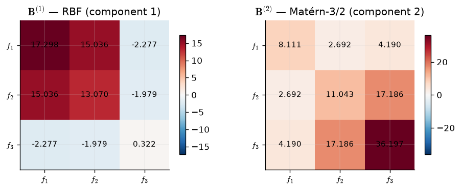
Fig. 32 Coregionalization matrices learned by the two LCM components, one paired with the RBF kernel and one with the Matérn-3/2 kernel.#
The two learned coregionalization matrices in Fig. 32 reveal the latent structure of the data. Each component has specialised: one captures the low-frequency correlations driven by \(g_1\), and the other captures the higher-frequency correlations driven by \(g_2\). Output 2, which depends on both latent functions, appears with non-negligible weight in both matrices — exactly as expected.
System configuration#
%reload_ext watermark
%watermark -n -u -v -iv -w -a 'Thomas Pinder'
Author: Thomas Pinder

Last updated: Fri, 07 Aug 2026

Python implementation: CPython
Python version       : 3.11.15
IPython version      : 9.15.0

gpjax     : 0.18.0
jax       : 0.10.2
jaxtyping : 0.3.11
matplotlib: 3.11.1

Watermark: 2.6.0